# Basefold

## Introduction

[**BaseFold**](https://eprint.iacr.org/2023/1705.pdf) is a new Polynomial Commitment Scheme that is field-agnostic, with verifier complexity of $$O(\log^2n)$$ and prover complexity of $$O(n \log n)$$. While the RS-code used in FRI-IOPP requires an FFT-friendly field, BaseFold eliminates this constraint by introducing the concept of **random foldable code**, making it usable with sufficiently large fields.

## Background

### Constant Polynomial in FRI-IOPP

In FRI, the following polynomial is folded using a random value $$\alpha\_0$$.

$$
P\_0(X) = c\_0 + c\_1X + c\_2X^2 + \cdots + c\_{2^k-1}X^{2^k-1}
$$

After the first round, the polynomial becomes:

$$
P\_1(X) = c\_0 + c\_1 \cdot \alpha\_0 + (c\_2 + c\_3 \cdot \alpha\_0) X + \cdots + (c\_{2^k-2} + c\_{2^k-1} \cdot\alpha\_0) X^{2^{k-1}- 1}
$$

If this folding process is repeated $$k+1$$ times, the resulting polynomial will eventually reduce to a constant polynomial, which looks like:

$$
P\_{k+1}(X) = c\_0 + c\_1\cdot \alpha\_0 + c\_2 \cdot \alpha\_1 + c\_3 \cdot \alpha\_1 \cdot \alpha\_0 + \cdots + c\_{2^k-1} \cdot \alpha\_0 \cdot \alpha\_1 \cdot \cdots \cdot \alpha\_k
$$

This constant polynomial is identical to the evaluation of the multilinear polynomial $$Q$$ at point $$(\alpha\_0, \alpha\_1, \alpha\_2, \dots, \alpha\_k)$$.

$$
Q(X\_0, X\_1, X\_2, \dots,X\_k) = c\_0+ c\_1X\_0 + c\_2X\_1 + \cdots + c\_{2^{k-1} -1}X\_0X\_1\cdots X\_{k}
$$

## Protocol Explanation

### Foldable Code

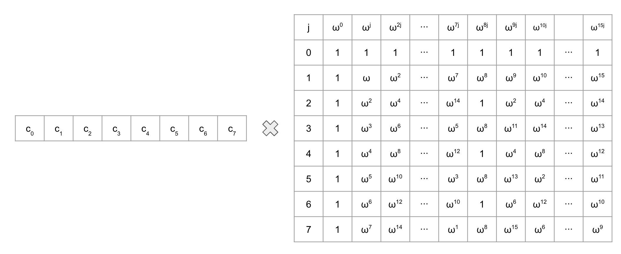
It is well-known that RS (Reed-Solomon) codes are a type of [linear code](https://en.wikipedia.org/wiki/Linear_code), and the encoding of linear codes can be represented as a matrix-vector multiplication. For example, the encoding of an $$\[n, k, d]$$-RS code, when $$n = 16$$ and $$k = 8$$, can be represented as follows:

<figure><img src="https://755218234-files.gitbook.io/~/files/v0/b/gitbook-x-prod.appspot.com/o/spaces%2Frwz1ZAZJtK5FHz4Y1esA%2Fuploads%2Fgit-blob-11943b0441296a9fc6f6348721460109e6b0ebfc%2FScreenshot%202024-12-23%20at%203.52.34%E2%80%AFPM.png?alt=media" alt=""><figcaption></figcaption></figure>

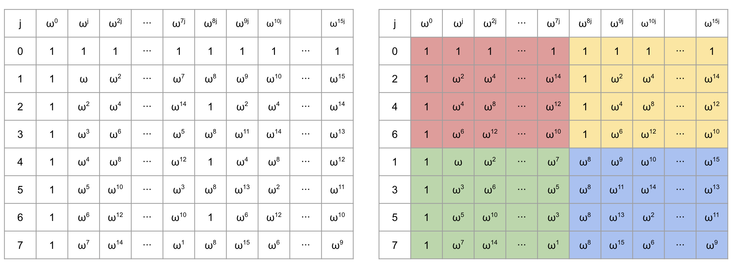
The matrix on the left can be transformed into the matrix on the right by applying a row permutation.

<figure><img src="https://755218234-files.gitbook.io/~/files/v0/b/gitbook-x-prod.appspot.com/o/spaces%2Frwz1ZAZJtK5FHz4Y1esA%2Fuploads%2Fgit-blob-e05968f0af5e67f4bd2d82f96904aa03789db995%2FScreenshot%202024-12-23%20at%203.57.32%E2%80%AFPM.png?alt=media" alt=""><figcaption></figcaption></figure>

If we divide the matrix on the right into four parts, the red and yellow-colored sections are identical and correspond to the matrix used in RS encoding when $$n = 8$$ and $$k = 4$$. The green-colored section is equivalent to multiplying the red matrix by a [diagonal matrix](https://en.wikipedia.org/wiki/Diagonal_matrix) $$T = \mathsf{diag}(1, \omega, \omega^2, \dots, \omega^7)$$. Similarly, the blue-colored section is equivalent to multiplying the red matrix by another diagonal matrix $$T' = \mathsf{diag}(\omega^8, \omega^9, \omega^{10}, \dots, \omega^{15})$$.

If the matrix used in the encoding of a linear code takes the form above, it is referred to as a **foldable** linear code. Let us define this more formally.

Let $$c, k\_0, d \in \mathbb{N}$$, $$k\_i = k\_0 \cdot 2^{i-1}, n\_i = c \cdot k\_i$$ for every $$i \in \[1,d]$$. A $$(c, k\_0,d)$$-**foldable linear code** is a [linear code](https://en.wikipedia.org/wiki/Linear_code) with a generator matrix $$G\_d$$ and rate $$\frac{1}{c}$$ with the following propertie&#x73;**:**

* the diagonal matrices $$T\_{i-1}, T'*{i-1} \in \mathbb{F}^{n*{i-1} \times n\_{i-1}}$$ satisfies that $$\mathsf{diag}(T\_{i-1})\[j] \ne \mathsf{diag}(T'*{i-1})\[j]$$ for every $$j \in \[0,n*{i-1}-1]$$.
* the matrix $$G\_i \in \mathbb{F}^{k\_i \times n\_i}$$ equals (up to row permutation)\\

$$
G\_i = \begin{bmatrix}
G\_{i−1} & G\_{i−1} \\
G\_{i−1} \cdot T\_{i-1} & G\_{i−1} \cdot T'\_{i-1} \\
\end{bmatrix}
$$

#### Random Foldable Code

To design a linear code that is foldable and efficiently encodable regardless of its finite field, BaseFold uses this algorithm:

1. Set $$G\_0 \leftarrow D\_0$$​, where $$D\_0$$​ is a distribution that outputs with 100% probability. Such a $$D\_i$$​ is referred to as a $$(c, k\_0)$$**-foldable distribution**.
2. Sample $$T\_i \leftarrow\_$ (\mathbb{F}^\times)^{n\_i}$$ and set $$T'\_i = -T\_i$$.
3. Generate $$G\_{i+1}$$​ using $$G\_i, T\_i, T'\_i$$.
4. Repeat steps 2 and 3 until a $$G\_i$$​ of the desired size is obtained.

This type of code is called a **Random Foldable Code (RFC)**. The paper demonstrates that this code has good relative minimum distance. For those interested, refer to Section 3.1 of the paper. Additionally, it is noted that this is a special case of punctured [Reed-Muller codes](https://en.wikipedia.org/wiki/Reed%E2%80%93Muller_code). For further details, consult Appendix D of the paper.

#### Encoding Algorithm

The encoding can be computed recursively as follows:

1. If $$i = 0$$, return $$\mathsf{Enc}\_0(m)$$.
2. Unpack $$1 \times k\_i$$ matrix $$m$$ into a pair of $$1 \times k\_i / 2$$ matrix $$(m\_l, m\_r)$$.
3. Set $$l = \mathsf{Enc}*{i-1}(m\_l)$$, $$t = \mathsf{diag}(T*{i-1})$$, and then pack a pair of $$k\_i  \times n\_i / 2$$ matrices $$(l + t \circ r, l - t \circ r)$$ to $$k\_i \times n\_i$$ matrix.

This approach is valid and can be proven inductively:

* If $$i = 0$$, $$\mathsf{Enc}\_0(m) = m \cdot G\_0$$​, which holds by definition.
* If $$i>0$$, $$\mathsf{Enc}\_i(m) = m \cdot G\_i$$ holds because of the recursive construction of $$G\_i$$.

$$
\begin{align\*}
l + t \circ r &= \mathsf{Enc}*{i-1}(m\_l) + \mathsf{diag}(T*{i-1}) \circ \mathsf{Enc}*{i-1}(m\_r) \\
&= m\_l \cdot G*{i-1} + \mathsf{diag}(T\_{d-1}) \circ (m\_r \cdot G\_{i-1}) \\
&= m\_l\cdot G\_{i-1} + m\_r \cdot G\_{i-1} \cdot T\_{i-1}
\end{align\*} \\

\begin{align\*}
l - t \circ r &= \mathsf{Enc}*{i-1}(m\_l)-  \mathsf{diag}(T*{i-1}) \circ \mathsf{Enc}*{i-1}(m\_r )\\
&= m\_l \cdot G*{i-1} - \mathsf{diag}(T\_{i-1}) \circ (m\_r \cdot G\_{i-1}) \\
&= m\_l\cdot G\_{i-1} - m\_r \cdot G\_{i-1} \cdot T\_{i-1}
\end{align\*} \\

(l+t\circ r, l-t \circ r) = (m\_l, m\_r) \cdot \begin{bmatrix}
G\_{i-1} \&G\_{i-1} \\
G\_{i-1} \cdot T\_{i-1} & G\_{i-1} \cdot -T\_{i-1}
\end{bmatrix} = m \cdot G\_i
$$

### BaseFold IOPP

To use this in IOPP, we need to ensure that $$\pi\_i$$ is indeed an encoded random linear combination derived from $$m\_{i+1}$$. To demonstrate this, let $$m\_i$$ ​represent the message at the $$i$$-th layer and $$\pi\_i$$ ​ the oracle (or block) at the $$i$$-th layer. Then, the following holds:

$$
\begin{align\*}
\pi\_{i+1} &= m\_{i+1}\cdot G\_{i+1} \\
&= m\_{i+1} \cdot \begin{bmatrix}
G\_i & G\_i \\
G\_i \cdot T\_i & G\_i \cdot T\_i'
\end{bmatrix} \\
&= \[\mathsf{Enc}*i(m*{i+1, l}) + \mathsf{diag}(T\_i) \circ \mathsf{Enc}*i(m*{i+1, r}) || \mathsf{Enc}*i(m*{i+1, l}) + \mathsf{diag}(T\_i') \circ \mathsf{Enc}*i(m*{i+1, r}) ]
\end{align\*}
$$

Thus, for $$j \in \[0, n\_i - 1]$$, the following conditions are satisfied, where $$n\_i$$ ​ is the length of $$\pi\_i$$:

$$
\pi\_{i+1}\[j] = \mathsf{Enc}*i(m*{i+1, l})\[j] + \mathsf{diag}(T\_i)\[j] \cdot \mathsf{Enc}*i(m*{i+1, r})\[j]  \\
\pi\_{i+1}\[j + n\_i] = \mathsf{Enc}*i(m*{i+1, l})\[j] + \mathsf{diag}(T\_i')\[j] \cdot \mathsf{Enc}*i(m*{i+1, r})\[j]
$$

The values $$\pi\_{i+1}\[j]$$ and $$\pi\_{i+1}\[j + n\_i]$$ are evaluations of the polynomial $$f(X) = \mathsf{Enc}*i(m*{i+1, l})\[j] + X \cdot \mathsf{Enc}*i(m*{i+1, r})\[j]$$ at $$\mathsf{diag}(T\_i)\[j]$$ and $$\mathsf{diag}(T\_i')\[j]$$, respectively. When using the sampled value $$\alpha\_i$$ at each $$i$$-th layer, $$f(\alpha\_i)$$ can be constructed as follows, ensuring that $$\pi\_i$$ encodes the message $$m\_{i,l} + \alpha\_i \cdot m\_{i, r}$$:

$$
\begin{align\*}
\pi\_i\[j] &= f(\alpha\_i) \\
&= \mathsf{Enc}*i(m*{i+1, l})\[j] + \alpha\_i \cdot \mathsf{Enc}*i(m*{i+1, r})\[j] \\
&=\mathsf{Enc}*i(m*{i+1, l} + \alpha\_i \cdot m\_{i+1, r})\[j]
\end{align\*}
$$

Using this property, an IOPP (Interactive Oracle Proof of Proximity) can be designed. Here, $$\text{interpolate}((x\_1, y\_1), (x\_2, y\_2))$$ refers to the computation of a degree-1 polynomial $$P$$ such that $$P(x\_1) = y\_1, P(x\_2) = y\_2$$.

$$\mathsf{IOPP.Commit}: \pi\_d := \mathsf{Enc}*d(f) \in \mathbb{F}^{n\_d} \rightarrow (\pi*{d - 1}, \dots, \pi\_0) \in \mathbb{F}^{n\_{d-1}} \times \cdots \times \mathbb{F}^{n\_0}$$

Prover witness: the polynomial $$f \in \mathbb{F}\[X\_0, X\_1, \dots, X\_{d-1}]$$

For $$i$$ from $$d − 1$$ to $$0$$:

1. The verifier samples $$\alpha\_i \leftarrow\_$ \mathbb{F}$$ and sends it to the prover.
2. For each index $$j \in \[0, n\_i - 1]$$, the prover
   1. sets $$f(X) := \mathsf{interpolate}((\mathsf{diag}(T\_i)\[j], π\_{i+1}\[j]),(\mathsf{diag}(T'*i)\[j], π*{i+1}\[j + n\_i]))$$.
   2. sets $$\pi\_i\[j] = f(\alpha\_i)$$.
3. The prover outputs oracle $$\pi\_i \in \mathbb{F}$$.

$$\mathsf{IOPP.Query}: (\pi\_d, \dots, \pi\_0) \rightarrow \text{accept or reject}$$

1. The verifier samples an index $$\mu \leftarrow\_$ \[0, n\_{d-1}-1]$$.
2. For $$i$$ from $$d − 1$$ to $$0$$, the verifier
   1. queries oracle entries $$\pi\_{i+1}\[\mu], \pi\_{i+1}\[\mu + n\_i]$$.
   2. computes $$p(X) := \mathsf{interpolate}((\mathsf{diag}(T\_i)\[\mu], π\_{i+1}\[\mu]),(\mathsf{diag}(T'*i)\[\mu], π*{i+1}\[\mu + n\_i]))$$.
   3. checks that $$p(α\_i) = \pi\_i\[\mu]$$.
   4. if $$i > 0$$ and $$\mu > n\_{i−1}$$, update $$\mu \leftarrow \mu − n\_{i−1}$$.
3. If $$\pi\_0$$ is a valid codeword w\.r.t. generator matrix $$G\_0$$, output **accept**, otherwise output **reject**.

### Multilinear PCS based on interleaving BaseFold IOPP

When performing the sumcheck protocol, the problem is reduced to an evaluation claim. Interestingly, the BaseFold IOPP shares a similar structure: given an input oracle that encodes a polynomial $$f \in \mathbb{F}\[X\_0, X\_1, \dots, X\_{d-1}]$$, the final oracle sent by the honest prover in the IOPP protocol is precisely an encoding of a random evaluation $$f(\bm{r})$$, where $$\bm{r} = (r\_0, r\_1, \dots, r\_{d-1})$$.

Thus, the sumcheck protocol and the IOPP protocol can be executed interleaved, sharing the same random challenge. At the end, the verifier needs to check whether the evaluation claim $$f(\bm{r})=y$$, obtained through the sumcheck protocol, matches the final prover message from the IOPP protocol. It performs as follows:

$$\mathsf{PC.Eval}$$

Public input: oracle $$\pi\_f := \mathsf{Enc}\_d(f) \in \mathbb{F}^{n\_d}$$, point $$\bm{r}$$, claimed evaluation $$y = f(\bm{r}) \in \mathbb{F}$$

Prover witness: the polynomial $$f \in \mathbb{F}\[X\_0, X\_1, \dots, X\_{d-1}]$$

1. The prover sends the following to the verifier:

$$
h\_d(X) =\sum\_{\bm{b} \in {0, 1}^{d-1}} f(\bm{b}, X) \cdot \widetilde{\mathsf{eq}}*r(\bm{b}, X), \\
\widetilde{\mathsf{eq}}*r(X\_0, X\_1, \dots, X*{d-1}) = \prod*{i = 0}^{d-1}(r\_i \cdot X\_i + (1 - r\_i)(1 - X\_i))
$$

3. For $$i$$ from $$d − 1$$ to $$0$$:
4. Verifier samples and sends $$r\_i \leftarrow\_$ \mathbb{F}$$ to the prover.
5. For each $$j \in \[0, n\_i - 1]$$, the prover
   1. sets $$g\_j(X) := \mathsf{interpolate}((\mathsf{diag}(T\_i)\[j], π\_{i+1}\[j]),(\mathsf{diag}(T'*i)\[j], π*{i+1}\[j + n\_i]))$$.
   2. sets $$\pi\_i\[j] = g\_j(r\_i)$$.
6. The prover outputs oracle $$\pi\_i ∈ \mathbb{F}^{n\_i}$$.
7. if $$i > 0$$, the prover sends verifier.

$$
h\_i(X) =\sum\_{\bm{b} \in {0, 1}^{i-1}} f(\bm{b}, X, r\_i, \dots, r\_{d-1}) \cdot \widetilde{\mathsf{eq}}*z(\bm{b}, X, r\_i, \dots, r*{d-1})
$$

8. The verifier checks that
   1. $$\mathsf{IOPP.query}^{(\pi\_d, \dots, \pi\_0)}$$ outputs accept.
   2. $$h\_d(0) + h\_d(1) \stackrel{?}= y$$ and for every $$i \in \[1, d - 1]$$, $$h\_i(0) + h\_i(1) \stackrel{?}= h\_{i+1}(r\_i)$$.
   3. $$\mathsf{Enc}\_0(h\_1(r\_0) / \widetilde{\mathsf{eq}}*z(r\_0, \dots, r*{d-1})) \stackrel{?}= \pi\_0$$.

## Conclusion

<figure><img src="https://755218234-files.gitbook.io/~/files/v0/b/gitbook-x-prod.appspot.com/o/spaces%2Frwz1ZAZJtK5FHz4Y1esA%2Fuploads%2Fgit-blob-776c42e787926dd16123212b42ad2aa1a33ae3a2%2Fimage.png?alt=media" alt=""><figcaption></figcaption></figure>

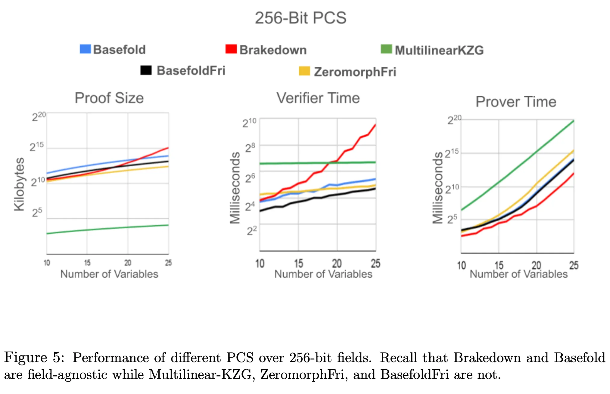
In a 256-bit PCS:

* BaseFold compared to field-agnostic Brakedown:
  * **Prover time**: Slower
  * **Verifier time**: Faster
  * **Proof size**: Bigger with a small number of variables but smaller with a large number of variables.
* BaseFoldFri compared to the non-field-agnostic ZeromorphFri:
  * **Prover time**: Faster
  * **Verifier time**: Faster
  * **Proof size**: Larger

<figure><img src="https://755218234-files.gitbook.io/~/files/v0/b/gitbook-x-prod.appspot.com/o/spaces%2Frwz1ZAZJtK5FHz4Y1esA%2Fuploads%2Fgit-blob-82391c5417ef27e8896f77979298798182d03df0%2Fimage.png?alt=media" alt=""><figcaption></figcaption></figure>

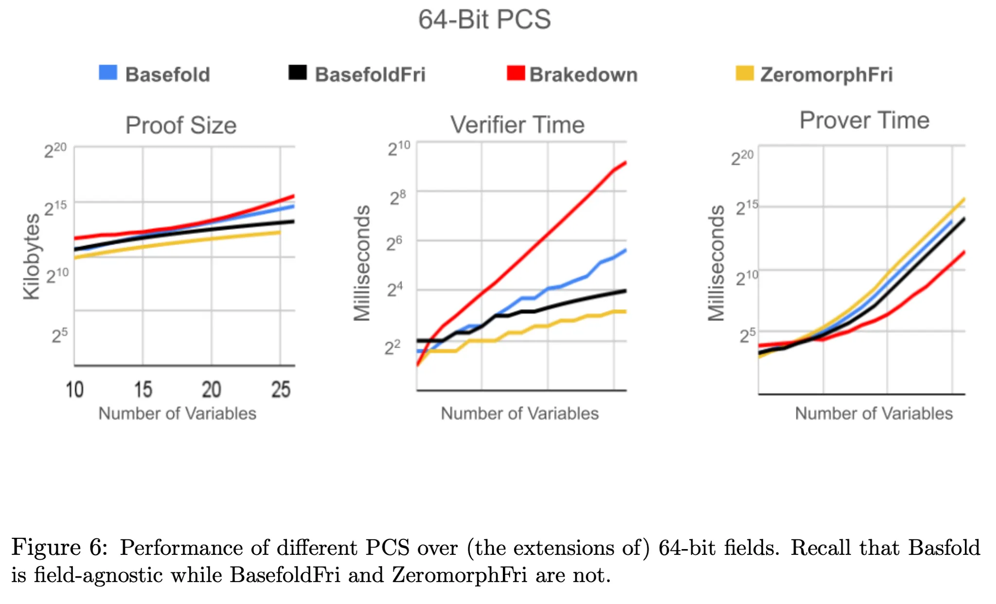
In a 64-bit PCS:

* BaseFold compared to field-agnostic Brakedown:
  * **Prover time**: Slower
  * **Verifier time**: Faster
  * **Proof size**: Smaller
* BaseFoldFri compared to the non-field-agnostic ZeromorphFri:
  * **Prover time**: Faster
  * **Verifier time**: Slower
  * **Proof size**: Larger

<figure><img src="https://755218234-files.gitbook.io/~/files/v0/b/gitbook-x-prod.appspot.com/o/spaces%2Frwz1ZAZJtK5FHz4Y1esA%2Fuploads%2Fgit-blob-fe0d63e3a380cd7c5c6494f13995cbdfa68c9413%2Fimage.png?alt=media" alt=""><figcaption></figcaption></figure>

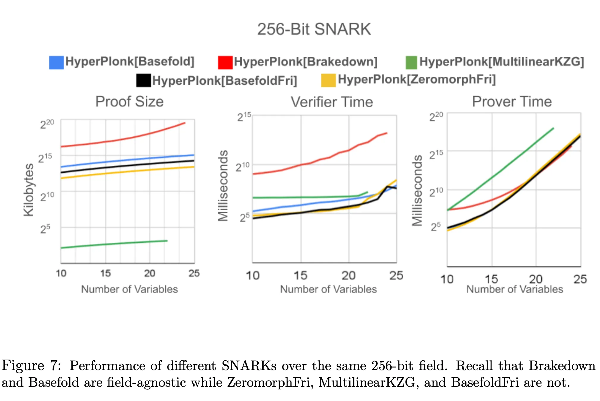
In a 256-bit SNARK:

* BaseFold compared to field-agnostic Brakedown:
  * **Prover time**: Faster with a small number of variables but similar with a large number of variables.
  * **Verifier time**: Faster
  * **Proof size**: Smaller
* BaseFoldFri compared to the non-field-agnostic ZeromorphFri:
  * **Prover time**: Similar
  * **Verifier time**: Similar
  * **Proof size**: Larger

<figure><img src="https://755218234-files.gitbook.io/~/files/v0/b/gitbook-x-prod.appspot.com/o/spaces%2Frwz1ZAZJtK5FHz4Y1esA%2Fuploads%2Fgit-blob-52cdfa565889e1c7772daf83175c7ccf4b386e96%2Fimage.png?alt=media" alt=""><figcaption></figcaption></figure>

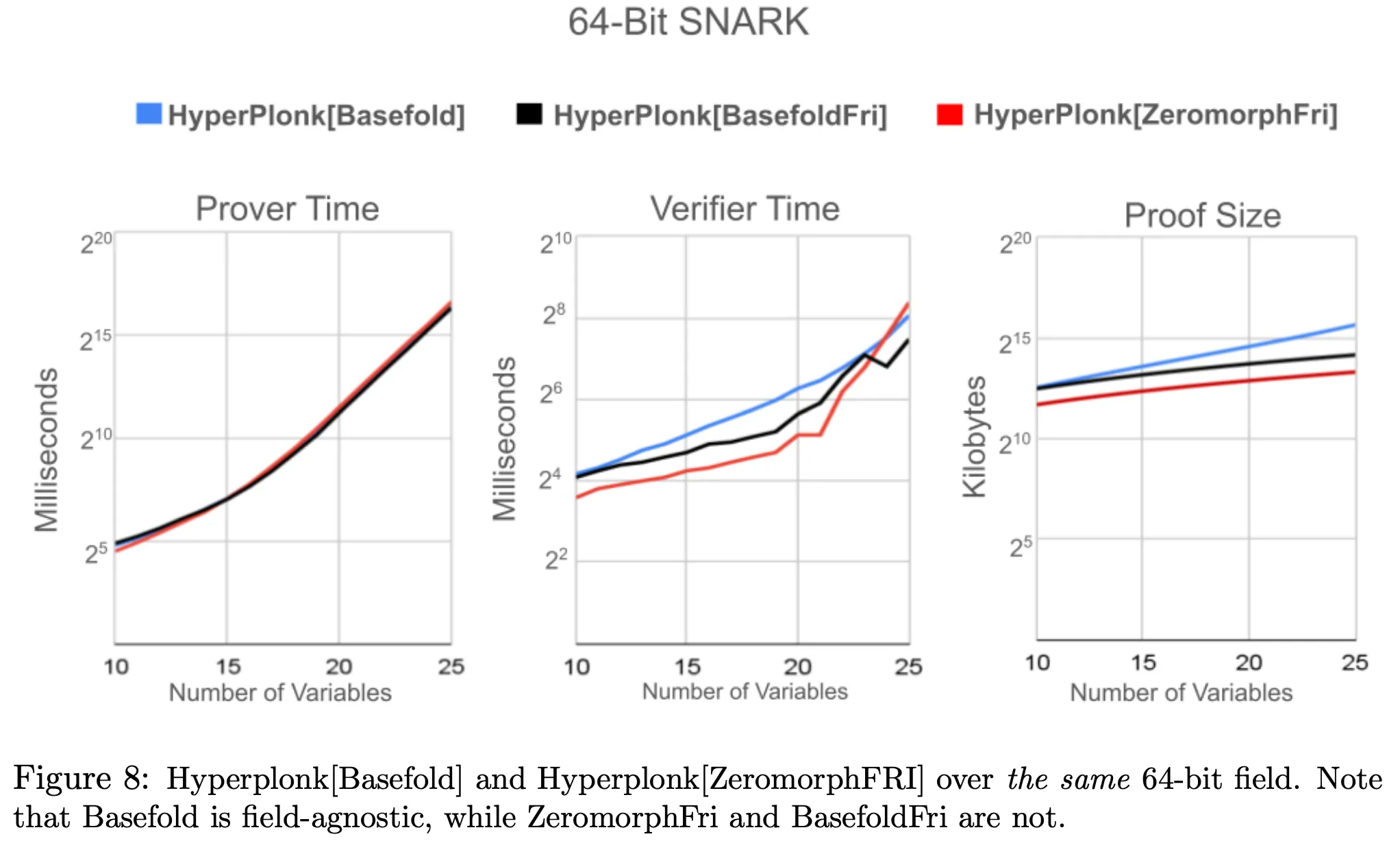
In a 64-bit SNARK:

* Both BaseFold and BaseFoldFri, compared to Zeromorph:
  * **Prover time**: Similar
  * **Verifier time**: Slower with a small number of variables but faster with a large number of variables.
  * **Proof size**: Larger

> Written by [Ryan Kim](https://app.gitbook.com/u/cPk8gft4tSd0Obi6ARBfoQ16SqG2 "mention") of Fractalyze