# Spartan
## Introduction
Various constructions for zkSNARKs over R1CS exist—[GGPR’s approach](https://eprint.iacr.org/2012/215.pdf), for instance, achieves $$O(n \log n)$$ proving time and $$O(1)$$ proof size, but requires a *per-statement* trusted setup with a large common reference string. Recent transparent zkSNARKs, such as Hyrax, STARK, Aurora, Ligero, and Bulletproofs, eliminate the need for trusted setups yet often impose limitations like circuit restrictions or linear verification costs. In Spartan, a new zkSNARK for arbitrary R1CS instances with sub-linear verification cost is introduced.
## Background
### Problem statement
Prior works are still lacking to achieve *truly* succinct SNARK without any trusted setup.
* The computational model of[ Hyrax](https://eprint.iacr.org/2017/1132.pdf) is layered arithmetic circuits, where the verifier’s costs and the proof sizes scale linearly in the depth of the circuit. For a depth-$$d$$ circuit, converting to a layered form increases the circuit size by a factor of $$O(d)$$, so Hyrax is restricted to low-depth circuits. Also, Hyrax achieves sublinear verification costs only for circuits with a uniform structure (e.g., data-parallel circuits).
* [STARK](https://eprint.iacr.org/2018/046.pdf) requires circuits with a sequence of identical sub-circuits, otherwise it does not achieve sublinear verification costs. Any circuit can be converted to this form, but the transformation increases circuit sizes by 10–1000×, which translates to a similar factor increase in the prover’s costs ([ref](https://eprint.iacr.org/2014/674.pdf)).
* [Ligero](https://eprint.iacr.org/2022/1608.pdf), [Bulletproofs](https://eprint.iacr.org/2017/1066.pdf), and [Aurora](https://eprint.iacr.org/2018/828.pdf) incur $$O(n)$$ verification costs.
So to summarize, there is two main challenges with achieving succinct verification:
1. Arbitrary circuits have no structure.
2. The verifier must know what statement is being proven. Because of these challenges, the verification must have complexity of at least $$O(|C|)$$ where $$|C|$$ implies circuit size.
**Spartan solution**: Verifier preprocesses the circuits - *without secret trapdoors to avoid any form of trusted setup.*
* Verifier retains a commitment to the circuit.
* Preprocessing incurs $$O(|C|)$$ costs but is amortized.
> The amortized cost here implies that even though the upfront computational or resource expense might be high, when spread over a large number of operations or over time, the average cost per operation becomes more manageable or efficient.
### Succinct interactive arguments of knowledge
From this paper, we adopt the notation $$\langle\mathcal{A}(z\_a),\mathcal{B}(z\_b)\rangle(x)$$ to denote the random variable representing the local output of machine $$\mathcal{B}$$ when interacting with the machine $$\mathcal{A}$$ on common input $$x$$, when the random tapes for each machine are uniformly and independently chosen, and $$\mathcal{A}$$ and $$\mathcal{B}$$ has auxiliary inputs $$z\_a$$ and $$z\_b$$, respectively.
Let $$\langle\mathcal{P},\mathcal{V}\rangle$$ denote a pair of [PPT](https://en.wikipedia.org/wiki/PP_\(complexity\)) algorithms and $$\mathsf{Setup}$$ denotes an algorithm that outputs public parameters $$\mathsf{pp}$$ given as input the security parameter $$\lambda$$.
[**Definition 2.5**](https://eprint.iacr.org/2019/550.pdf#page=9\&zoom=100,178,200) **from the paper**. A protocol between a pair of [PPT](https://en.wikipedia.org/wiki/PP_\(complexity\)) algorithms $$\langle\mathcal{P},\mathcal{V}\rangle$$ is called a public-coin succinct interactive argument of knowledge for a language $$\mathcal{L}$$ if:
* **Completeness**. For any problem instance $$\mathbf{x}\in\mathcal{L}$$, there exists a witness $$w$$ such that for all $$r\in{0, 1}^{\*}$$, $$\mathsf{Pr}{\langle\mathcal{P}(\mathsf{pp},w),\mathcal{V}(\mathsf{pp},r)\rangle(\mathbf{x}) = 1} ≥ 1 − \mathsf{negl}(\lambda)$$.
* **Soundness**. For any non-satisfiable problem instance $$\mathbf{x}$$, any PPT prover $$P^∗$$ , and for all $$w,r\in{0, 1}^∗$$, $$Pr{\langle\mathcal{P}^\* (\mathsf{pp},w), \mathcal{V}(\mathsf{pp},r)⟩(\mathbf{x}) = 1} ≤ \mathsf{negl}(\lambda)$$.
* **Knowledge soundness**. For any PPT adversary $$\mathcal{A}$$, there exists a PPT extractor $$\mathcal{E}$$ such that for any problem instance $$\mathbf{x}$$ and for all $$w,r\in{0, 1}^∗$$ , if $$\mathsf{Pr}{\langle\mathcal{A}(pp, w), \mathcal{V}(\mathsf{pp},r)⟩(\mathbf{x}) = 1} \geq\mathsf{negl}(\lambda)$$, then $$\mathsf{Pr}{\mathsf{Sat}\_\mathcal{L}(\mathbf{x},w') = 1|w'\leftarrow\mathcal{E}^{\mathcal{A}}(\mathsf{pp}, \mathbf{x})} \geq \mathsf{negl}(\lambda)$$.
* **Succinctness**. The total communication between $$\mathcal{P}$$ and $$\mathcal{V}$$ is sublinear in the size of the NP statement $$\mathbf{x}\in\mathcal{L}$$.
* **Public coin**. $$\mathcal{V}$$'s messages are chosen uniformly at random.
### The sumcheck protocol
Using [sumcheck](https://fractalyze.gitbook.io/intro/~/revisions/GBuVDfZJZBNDtoleSgnx/primitives/sumcheck), a prover can prove statements of the form:
$$
\sum\_{\bm{x}\in{0,1}^\mu}\mathcal{G}(\bm{x})\stackrel{?}{=}T
$$
We can denote the sumcheck protocol as $$\mathsf{IsSat}\leftarrow\langle\mathcal{P}*{sc},\mathcal{V}*{sc}(\bm{r})\rangle(\mathcal{G},\mu,l,T)$$ for any $$\mu$$-variate polynomial $$\mathcal{G}$$ with degree at most $$l$$ in each variable. This is typically reduced to the claim $$\mathcal{G}(\bm{r})\stackrel{?}{=}e$$ and using $$\mu$$ round interactive protocol which can be denoted as $$e\leftarrow\langle\mathcal{P}*{sc}(\mathcal{G}),\mathcal{V}*{sc}(\bm{r})\rangle(\mu,l,T)$$
This proof system does not require a trusted setup. It can be made zero-knowledge and non-interactive with existing compilers but still cannot be used as a zkSNARK. The main two reasons for this are:
1. We need an efficient reduction from R1CS statements to sumcheck instances.
2. The proof system is not succinct (both proof sizes and verification times).
1. Generally, the verifier must evaluate $$\mathcal{G}$$ at some random point in its domain $$\bm{r}=(r\_1,\dots,r\_\mu)$$.
### Multilinear polynomial extension
[**Definition 2.8**](https://eprint.iacr.org/2019/550.pdf#page=10\&zoom=100,178,350)**. (Multilinear polynomial)** A multivariate polynomial is called a multilinear polynomial if the degree of the polynomial in each variable is at most one.
[**Definition 2.9**](https://eprint.iacr.org/2019/550.pdf#page=10\&zoom=100,178,390)**. (Low-degree polynomial)** A multivariate polynomial $$\mathcal{G}$$ over a finite field $$\mathbb{F}$$ is called low-degree polynomial if the degree of $$\mathcal{G}$$ in each variable is exponentially smaller than $$|\mathbb{F}|$$.
**Low-degree extensions (LDEs).** Suppose $$g:{0,1}^\mu\rightarrow\mathbb{F}$$ is a function that maps $$\mu$$-bit elements into an element of $$\mathbb{F}$$. A polynomial extension of $$g$$ is a low-degree $$\mu$$-variate polynomial $$\tilde{\mathcal{g}}(\cdot)$$ such that $$\tilde{\mathcal{g}}(\bm{x})=\mathcal{g}(\bm{x})$$ for all $$\bm{x}\in{0,1}^\mu$$.
**Multilinear extension (MLE)** is a LDE where the extension is a multilinear polynomial. Given a function $$Z:{0,1}^\mu\rightarrow\mathbb{F}$$, the MLE of $$Z(\cdot)$$ is the unique multilinear polynomial $$\tilde{Z}:\mathbb{F}^\mu\rightarrow\mathbb{F}$$. It can be computed as follows:
$$
\widetilde{Z}(x\_1,\dots,x\_\mu)=\sum\_{\bm{e}\in{0,1}^m}Z(\bm{e})\cdot \prod\_{i=1}^\mu(x\_i\cdot e\_i + (1-x\_i)\cdot (1-e\_i) \ = \sum\_{\bm{e}\in{0,1}^\mu}Z(\bm{e})\cdot \widetilde{\mathsf{eq}}(\bm{x},\bm{e})
$$
Note that $$\widetilde{\mathsf{eq}}(\bm{x},\bm{e})$$ is the MLE of the following function:
$$
\mathsf{eq}(\bm{x},\bm{e})=
\begin{cases}
1 &\text{if}\ \bm{x}=\bm{e} & \\
0 & \text{otherwise}
\end{cases}
$$
> For any $$\bm{r}\in \mathbb{F}^\mu$$, $$\tilde{Z}(\bm{r})$$ can be computed in $$O(2^\mu)$$ operations in $$\mathbb{F}$$. \[[96](https://ieeexplore.ieee.org/stamp/stamp.jsp?tp=\&arnumber=6547112), [99](https://eprint.iacr.org/2013/351.pdf)]
### Polynomial commitment scheme for multilinear polynomials
A polynomial commitment scheme for multilinear polynomials is a tuple of four protocols $$\mathsf{PC} = (\mathsf{Setup}, \mathsf{Commit}, \mathsf{Open}, \mathsf{Eval})$$.
* $$\mathsf{pp} \leftarrow \mathsf{Setup}(1^λ, \mu)$$: takes as input $$\mu$$ (the number of variables in a multilinear polynomial); produces public parameters $$\mathsf{pp}$$.
* $$(\mathcal{C}; \mathcal{S}) \leftarrow \mathsf{Commit}(\mathsf{pp}; \mathcal{G})$$: takes as input a $$\mu$$-variate multilinear polynomial over a finite field $$\mathcal{G} \in \mathbb{F}\[X\_1,...,X\_\mu]$$; produces a public commitment $$\mathcal{C}$$ and a secret opening hint $$\mathcal{S}$$.
* $$b \leftarrow \mathsf{Open}(\mathsf{pp}, \mathcal{C}, \mathcal{G}, \mathcal{S})$$: verifies the opening of commitment $$\mathcal{C}$$ to the $$\mu$$-variate multilinear polynomial $$\mathcal{G} \in \mathbb{F}\[X\_1,\dots,X\_\mu]$$ with the opening hint $$\mathcal{S}$$; outputs a boolean $$b \in {0, 1}$$.
* $$b \leftarrow \mathsf{Eval}(\mathsf{pp}, \mathcal{C}, r, v; \mathcal{G}, \mathcal{S})$$ is an interactive public-coin protocol between a [PPT](https://en.wikipedia.org/wiki/PP_\(complexity\)) prover $$\mathcal{P}$$ and verifier $$\mathcal{V}$$. Both $$\mathcal{V}$$ and $$\mathcal{P}$$ hold a commitment $$\mathcal{C}$$, a scalar $$v\in\mathbb{F}$$ , and $$r\in \mathbb{F}^\mu$$. $$\mathcal{P}$$ additionally knows a $$\mu$$-variate multilinear polynomial $$\mathcal{G} \in\mathbb{F} \[X\_1,\dots,X\_\mu]$$ and its secret opening hint $$\mathcal{S}$$. $$\mathcal{P}$$ attempts to convince $$\mathcal{V}$$ that $$\mathcal{G}(r) = v$$. At the end of the protocol, $$\mathcal{V}$$ outputs $$b \in {0, 1}$$.
## Protocol Explanation
### R1CS as a multivariate function
[**Theorem 4.1**](https://eprint.iacr.org/2019/550.pdf#page=16\&zoom=100,178,620) **from the paper.** For any R1CS instance $$\mathbf{x}=(\mathbb{F},\bm{A,B,C},\bm{io},m,n)$$ there exists a degree-3, $$\log m$$-variate polynomial $$\mathcal{G}$$ such that $$\sum\_{\bm{x}\in{0,1}^{\log m}}\mathcal{G}(\bm{x})=0$$ if and only if there exists a witness $$w$$ such that $$\mathsf{Sat}(\mathbb{x},w)=1$$ (except for a soundness error that is negligible in $$\lambda$$). Here, $$n$$ is the upper bound on the non-zero entries in the $$\bm{A}, \bm{B}, \bm{C}$$ matrices.
If we denote $$\log m = s$$ for the sake of simplicity, for a given $$\bm{A,B,C}\in\mathbb{F}^{m\times m}$$, we can view them as functions with the following signature: $${0,1}^s\times{0,1}^s\rightarrow \mathbb{F}$$. Furthermore, given a witness $$\bm{w}$$ to instance $$\mathbf{x}$$, let $$\bm{Z}=(\bm{io},1,\bm{w})$$. Then we can also view $$\bm{Z}$$ as a function mapping $${0,1}^s\rightarrow\mathbb{F}$$.
We define $$F\_{\bm{io}}(\cdot)$$ that can be used to encode $$\bm{w}$$ as:
$$
F\_{\bm{io}}(\bm{x})=\sum\_{\bm{y}\in{0,1}^s}A(\bm{x,y})Z(\bm{y})\cdot\sum\_{\bm{y}\in{0,1}^s}B(\bm{x,y})Z(\bm{y}) -\ - \sum\_{\bm{y}\in{0,1}^s}C(\bm{x,y})Z(\bm{y})
$$
[**Lemma 4.1**](https://eprint.iacr.org/2019/550.pdf#page=17\&zoom=100,178,265) **from the paper.** $$\forall \bm{x}\in{0,1}^s, F\_{io}(x)=0$$ if and only if $$\mathsf{Sat}(\mathbf{x},\bm{w})=1$$.
> Proof. This follows from the definition of $$\mathsf{Sat}\_\mathsf{R1CS}(\mathbf{x}, \bm{w})$$ (Section 2.1) and of $$Z(\cdot)$$. $$\square$$
### Functions to polynomials
Unfortunately, $$F\_{io}(\cdot)$$ is a function, *not* a polynomial, so it cannot be directly used in the sumcheck protocol. But, consider its polynomial extension $$\tilde{F}\_{\bm{io}}:\mathbb{F}^s\rightarrow\mathbb{F}$$:
$$
\tilde{F}*{\bm{io}}(\bm{x})=\sum*{\bm{y}\in{0,1}^s}\tilde{A}(\bm{x,y})\tilde{Z}(\bm{y})\sum\_{\bm{y}\in{0,1}^s}\tilde{B}(\bm{x,y})\tilde{Z}(\bm{y}) - \ - \sum\_{\bm{y}\in{0,1}^s}\tilde{C}(\bm{x,y})\tilde{Z}(\bm{y})
$$
[**Lemma 4.2**](https://eprint.iacr.org/2019/550.pdf#page=17\&zoom=100,178,425) **from the paper.** Then, $$\forall \bm{x}\in{0,1}^s, \tilde{F}\_{\bm{io}}(\bm{x})=0$$ if and only if $$\mathsf{Sat}(\mathbf{x},\bm{w})=1$$.
> Proof. For any $$\bm{x} \in {0, 1}^s$$, $$\tilde{F}*{\bm{io}}(x) = F*{\bm{io}}(x)$$, so the result follows from Lemma 4.1. $$\square$$
Since $$\tilde{F}*{\bm{io}}(\cdot)$$ is a low-degree multivariate polynomial over $$\mathbb{F}$$ in $$s$$ variables, a verifier could check if $$\sum*{\bm{x}\in{0,1}^s}\tilde{F}\_{\bm{io}}(\bm{x})=0$$ using the sumcheck protocol. But the sum being 0 doesn't exactly mean that each of them was 0 since some of the terms in the sum may cancel each other out. This is addressed using a prior idea from [LegoSNARK](https://eprint.iacr.org/2019/142.pdf) by taking:
$$
\mathcal{G}*{\bm{io},\tau}(\bm{x})=\tilde{F}*{\bm{io}}(\bm{x})\cdot\widetilde{\mathsf{eq}}(\bm{\tau},\bm{x})
$$
$$
Q\_{\bm{io}}(\bm{\tau})=\sum\_{\bm{x}\in{0,1}^s}\mathcal{G}*{\bm{io},\bm{\tau}}(\bm{x})=\sum*{\bm{x}\in{0,1}^s}\tilde{F}\_{\bm{io}}(\bm{x})\cdot\widetilde{\mathsf{eq}}(\bm{\tau},\bm{x})
$$
Observe that:
* $$Q\_{\bm{io}}$$ is same as $$\tilde{F}*{\bm{io}}$$ over the boolean hypercube*.\_
* $$Q\_{\bm{io}}$$ is $$s$$-variate multilinear polynomial
* $$\forall\bm{t}\in{0,1}^s$$, $$Q\_{\bm{io}}(\bm{t})=0 \Leftrightarrow \mathsf{Sat}(\mathbf{x},\bm{w})=1$$ . Therefore, Since it has $$2^s$$ solutions, it has to be a 0 polynomial over the $$\mathbb{F}^s$$ if and only if $$\mathsf{Sat(\mathbf{x},\bm{w})}=1$$.
This implies that $$Q\_{\bm{io}}(\bm{\tau})$$ is zero-polynomial if and only if $$\mathsf{Sat}(\mathbb{x},w)=1$$ and to check if $$Q\_{\bm{io}}(\cdot)$$ is a zero-polynomial, its enough with a single random challenge $$Q\_{\bm{io}}(\bm{r\_\tau})\stackrel{?}{=}0$$ where $$\bm{r\_\tau}\in\_R \mathbb{F}^s$$ (this will introduce soundness error $$\frac{\log m}{|\mathbb{F}|})$$.
**Proof of** [**Theorem 4.1**](https://eprint.iacr.org/2019/550.pdf#page=16\&zoom=100,178,620). For a given R1CS instance $$\mathbf{x} = (\mathbb{F} ,\bm{A},\bm{B},\bm{C}, \bm{io}, m, n)$$, define, $$\mathcal{G}*{\bm{io},\bm{\tau}} (\bm{x}) = \tilde{F}*{\bm{io}}(\bm{x}) \cdot\widetilde{\mathsf{eq}}(\bm{\tau}, \bm{x})$$, so $$Q\_{io}(\bm{\tau}) = \sum\_{\bm{x}∈{0,1}^s}\mathcal{G}*{\bm{io},\bm{\tau}}(\bm{x})$$. Observe that $$\mathcal{G}*{\bm{io},\bm{\tau}}(\cdot)$$ is a degree-3 $$s$$-variate polynomial if multilinear extensions of $$\bm{A},\bm{B},\bm{C}$$, and $$\bm{Z}$$ are used in $$\tilde{F}*{\bm{io}}(\cdot)$$. In the terminology of the sumcheck protocol, $$T = 0$$, $$\mu = s = \log m$$, and $$l = 3$$. Furthermore, if $$\bm{r*\tau}\in\_R\mathbb{F}^s$$, $$\sum\_{\bm{x}\in{0,1}^s} \mathcal{G}*{\bm{io},\bm{r*\tau}} (\bm{x}) = 0$$ if and only $$\tilde{F}\_{\bm{io}}(\bm{x}) = 0$$, $$\forall \bm{x}\in{0,1}^s$$—except for soundness error that is negligible in $$\lambda$$ under the assumptions noted above ([Lemma 4.3](https://eprint.iacr.org/2019/550.pdf#page=17\&zoom=100,178,770)). This combined with [Lemma 4.2](https://eprint.iacr.org/2019/550.pdf#page=17\&zoom=100,178,425) implies the desired result.
[**Theorem 5.1** ](https://eprint.iacr.org/2019/550.pdf#page=18\&zoom=100,178,370)**from the paper**. Given an extractable polynomial commitment scheme for multilinear polynomials, there exists a public-coin succinct interactive argument of knowledge where security holds under the assumptions needed for the polynomial commitment scheme and assuming $$|\mathbb{F}|$$ is exponential in $$\lambda$$ and the size parameter of R1CS instance $$n = O(\lambda)$$.
[Theorem 4.1 ](https://eprint.iacr.org/2019/550.pdf#page=16\&zoom=100,178,620)established that for $$\mathcal{V}$$ to verify if an R1CS instance $$\mathbf{x}=(\mathbb{F},\bm{A,B,C},\bm{io},m,n)$$ is satisfiable, it can check if $$\sum\_{\bm{x}\in{0,1}^{\log m}}\mathcal{G}*{\bm{io},\bm{\tau}}(\bm{x})=0$$. By using the sumcheck protocol, we can reduce the claim about the sum to $$e\_x \stackrel{?}{=} \mathcal{G}*{\bm{io},\bm{\tau}}(\bm{r}\_x)$$ where $$\bm{r}*x\in \mathbb{F}^s$$, so $$\mathcal{V}$$ needs a mechanism to evaluate $$\mathcal{G}*{\bm{io},\bm{\tau}}(\bm{r}\_x)$$—without incurring $$O(m)$$ communication from $$\mathcal{P}$$ to $$\mathcal{V}$$.
So let's denote it as the following:
$$
\displaylines{\bar{A}(r\_x)=\sum\_{y\in{0,1}^s}\tilde{A}(r\_x,y)\cdot\tilde{Z}(y) \newline \bar{B}(r\_x)=\sum\_{y\in{0,1}^s}\tilde{B}(r\_x,y)\cdot\tilde{Z}(y)\newline \bar{C}(r\_x)=\sum\_{y\in{0,1}^s}\tilde{C}(r\_x,y)\cdot\tilde{Z}(y)}
$$
Now, the prover can make three separate claims $$\bar{A}(\bm{r}\_x)=v\_A, \bar{B}(\bm{r}\_x)=v\_B, \bar{C}(\bm{r}\_x)=v\_C$$ and verifier can check:
$$
\mathcal{G}\_{io,\tau}(\bm{r}\_x)=(v\_A\cdot v\_B - v\_C)\cdot\widetilde{\mathsf{eq}}(r\_x,\tau)\stackrel{?}=e\_x
$$
Of course, the verifier still needs verify the $$v\_A, v\_B, v\_C$$ claims and to do so, it can run three independent instances of sumcheck protocol but instead, we can use a [prior idea](https://eprint.iacr.org/2017/1132.pdf) to combine these into a single claim:
1. Verifier samples $$r\_A, r\_B, r\_C \leftarrow \mathbb{F}$$ and computes $$c=r\_A\cdot v\_A + r\_B\cdot v\_B + r\_C \cdot v\_C$$.
2. Let $$L(\bm{x})=r\_A\cdot\bar{A}(\bm{x}) + r\_B\cdot\bar{B}(\bm{x})+r\_C\cdot\bar{C}(\bm{x})$$. Then:
$$
L(\bm{r}*x)=\sum*{\bm{y}\in{0,1}^s}r\_A\cdot\tilde{A}(\bm{r}\_x,\bm{y})\tilde{Z}(\bm{y})+r\_B\cdot\tilde{B}(\bm{r}*x,\bm{y})\tilde{Z}(\bm{y}) +r\_C\cdot\tilde{C}(\bm{r}*x,\bm{y})\tilde{Z}(\bm{y}) \ = \sum*{\bm{y}\in{0,1}^s}\bm{M}*{\bm{r}\_x}(\bm{y})
$$
3. Verifier uses sumcheck to verify:
$$
r\_A\cdot\bar{A}(r\_x) + r\_B\cdot\bar{B}(r\_x)+r\_C\cdot\bar{C}(r\_x)=\sum\_{\bm{y}\in{0,1}^s}\bm{M}\_{\bm{r}\_x}(\bm{y})\stackrel{?}{=}c
$$
Still there are some problems left. To verify the last sumcheck $$\sum\_{\bm{y}\in{0,1}^s}\bm{M}\_{\bm{r}*x}(\bm{y})\stackrel{?}{=}c$$, the verifier has to evaluate $$\bm{M}*{\bm{r}\_x}$$ at some random $$\bm{r}\_y\in\_R \mathbb{F}^s$$:
$$
\bm{M}\_{\bm{r}\_x}(\bm{r}\_y)=r\_A\cdot\tilde{A}(\bm{r}\_x,\bm{r}\_y)\tilde{Z}(\bm{r}\_y)+r\_B\cdot\tilde{B}(\bm{r}\_x,\bm{r}\_y)\tilde{Z}(\bm{r}\_y) +r\_C\cdot\tilde{C}(\bm{r}\_x,\bm{r}\_y)\tilde{Z}(\bm{r}\_y) \ =(r\_A\cdot\tilde{A}(\bm{r}\_x,\bm{r}\_y)+r\_B\cdot\tilde{B}(\bm{r}\_x,\bm{r}\_y) +r\_C\cdot\tilde{C}(\bm{r}\_x,\bm{r}\_y))\cdot\tilde{Z}(\bm{r}\_y)
$$
Observe that the only term in $$\bm{M}\_{\bm{r}\_x}(\bm{r}\_y)$$ that depends on the prover’s witness is $$\tilde{Z}(\bm{r}\_y)$$. This is because all other terms in the above expression can be computed locally by $$\mathcal{V}$$ using $$\mathbf{x}=(\mathbb{F},\bm{A,B,C},\bm{io},m,n)$$ in $$O(n)$$ time ([Section 6](https://eprint.iacr.org/2019/550.pdf#page=22\&zoom=100,178,340) in the paper discusses how to reduce the cost of those evaluations to be sub-linear in $$n$$).
To evaluate $$\tilde{Z}(\bm{r}\_y)$$, $$\mathcal{V}$$ does the following. WLOG, assume $$|\bm{w}| = |\bm{io}| + 1$$. Thus, by the closed form expression of multilinear polynomial evaluations, we have:
$$
\tilde{Z}(\bm{r}\_y)=\bm{r}\_y\[0]\cdot\tilde{w}(\bm{r}\_y\[1..]) + (1-\bm{r}\_y\[0])\cdot\widetilde{(\bm{io},1)} (\bm{r}\_y\[1..])
$$
If you recall that $$\bm{Z}=(\bm{io},1,\bm{w})$$ and $$\widetilde{\mathsf{eq}}(\bm{e},\bm{x})=\prod\_{i=1}^s(x\_i\cdot e\_i + (1-x\_i)(1-e\_i))$$:
$$
\tilde{Z}(x\_1,\dots,x\_s)=\sum\_{\bm{e}\in{0,1}^s}Z(\bm{e})\cdot \widetilde{\mathsf{eq}}(\bm{e},\bm{x}) \\=x\_1\cdot \sum\_{\bm{e'}\in{0,1}^{s-1}}Z(1,\bm{e'})\cdot \widetilde{\mathsf{eq}}(\bm{e'},\bm{x}\[1..]) + \ +(1-x\_1)\cdot \sum\_{\bm{e'}\in{0,1}^{s-1}}Z(0,\bm{e'})\cdot \widetilde{\mathsf{eq}}(\bm{e'},\bm{x}\[1..])\ = x\_1 \cdot \tilde{w}(\bm{x}\[1..])+(1-x\_1)\cdot\widetilde{(\bm{io},1})(\bm{x}\[1..])
$$
Similar technique is also used by [vSQL](https://www.ieee-security.org/TC/SP2017/papers/581.pdf) under the section [*Avoiding Relaying the Inputs*](https://www.ieee-security.org/TC/SP2017/papers/581.pdf#page=11\&zoom=100,50,450)*.*
### Putting them together for NIZK
We assume that there exists an extractable polynomial commitment scheme for multilinear polynomials $$\mathsf{PC}=(\mathsf{Setup, Commit, Open, Eval)}$$.
* $$\mathsf{pp}\leftarrow \mathsf{PC.Setup}(1^\lambda,s)$$
* $$\mathsf{IsSat}\leftarrow\langle\mathcal{P}(\bm{w}),\mathcal{V}(r)\rangle(\mathbb{F},\bm{A},\bm{B},\bm{C},\bm{io},m,n):$$
1. $$\mathcal{P}:(\mathcal{C},\mathcal{S})\leftarrow \mathsf{PC.Commit}(\mathsf{pp},\tilde{\bm{w}})$$ and send $$\mathcal{C}$$ to $$\mathcal{V}$$.
2. $$\mathcal{V}:\bm{\tau}\in\_R\mathbb{F}^{s}$$ and send $$\bm{\tau}$$ to $$\mathcal{P}$$
3. Let $$T\_1=0, \mu\_1=\log m,l\_1=3$$.
4. $$\mathcal{V}:$$ Sample $$\bm{r}\_x\in\_R\mathbb{F}^{\mu\_1}$$
5. **Sumcheck #1:** $$e\_x\leftarrow\langle\mathcal{P}*{sc}(\mathcal{G}*{\bm{io},\bm{\tau}}),\mathcal{V}\_{sc}(\bm{r}\_x)\rangle(\mu\_1,l\_1,T\_1)$$
6. $$\mathcal{P}:$$ Compute $$\bar{A}(\bm{r}\_x)=v\_A, \bar{B}(\bm{r}\_x)=v\_B, \bar{C}(\bm{r}\_x)=v\_C$$ and send $$(v\_A,v\_B,v\_C)\rightarrow \mathcal{V}$$.
7. $$\mathcal{V}:$$ Abort with $$\mathsf{IsSat}=0$$ if $$e\_x\neq(v\_A\cdot v\_B - v\_C)\cdot\tilde{eq}(\bm{r}\_x,\bm{\tau}).$$
8. $$\mathcal{V}:$$ Sample $$r\_A,r\_B,r\_C\in\_R\mathbb{F}$$ and send them to $$\mathcal{P}$$.
9. Let $$T\_2=r\_A\cdot v\_A + r\_B\cdot v\_B + r\_C\cdot v\_C, \mu\_2=\log m, l\_2=2$$.
10. $$\mathcal{V}:$$ Sample $$r\_y\in\_R \mathbb{F}^{\mu\_2}$$
11. **Sumcheck #2:** $$e\_y\leftarrow\langle\mathcal{P}*{sc}(\bm{M}*{\bm{r}*x}),\mathcal{V}*{sc}(\bm{r}\_y)\rangle(\mu\_2,l\_2,T\_2)$$
12. $$\mathcal{P} : v\leftarrow \tilde{w}(r\_y\[1..])$$ and send $$v$$ to $$\mathcal{V}$$.
13. $$\mathsf{IsSat}*e \leftarrow \langle\mathcal{P}*\mathsf{PC.Eval}(\tilde{w},\mathcal{S}),\mathcal{V}\_\mathsf{PC.Eval}(r)\rangle(\mathsf{pp}, \mathcal{C},r\_y\[1..],v,\mu\_2)$$
14. $$\mathcal{V}:$$ if $$\mathsf{IsSat}\_e == 0$$, abort with $$\mathsf{IsSat}=0$$.
15. $$\mathcal{V}: v\_Z\leftarrow r\_y\[0]\cdot v+(1-r\_y\[0])\cdot\widetilde{(\bm{io},1)}(r\_y\[1...])$$
16. $$\mathcal{V}:v\_1\leftarrow\tilde{A}(r\_x,r\_y),v\_2\leftarrow\tilde{B}(r\_x,r\_y),v\_3\leftarrow\tilde{C}(r\_x,r\_y)$$
17. $$\mathcal{V}:$$ Abort with $$\mathsf{IsSat}=0$$ if $$e\_y\neq(r\_A\cdot v\_1 + r\_B\cdot v\_2 + r\_C\cdot v\_3)\cdot v\_Z$$
18. $$\mathcal{V}:$$ return $$\mathsf{IsSat}=1$$
#### Cost Analysis
List of possible PCS schemes that can be used
* Prover:
* $$O(n)$$ for each sumcheck instances
* Cost of $$\mathsf{PC.Commit}$$ and $$\mathsf{PC.Eval}$$ for $$\log m$$-variate multilinear polynomial $$\tilde{w}(\cdot)$$.
* Verifier:
* $$O(\log m)$$ for each sumcheck instances
* Cost of $$\mathsf{PC.Eval}$$ for $$log\ m$$-variate multilinear polynomial $$\tilde{w}(\cdot)$$
* $$O(n)$$ to evaluate $$\tilde{A}, \tilde{B}, \tilde{C}$$ at $$(\bm{r}\_x, \bm{r}\_y)$$
* Communication cost:
* $$O(\log m)$$ for each sumcheck instances
* The size of the commitment to $$\tilde{w}(\cdot)$$ and the communication in $$\mathsf{PC.Eval}$$
Total cost of the SpartanNIZK depending on PCS choice
### Computation commitments: zkSNARK from NIZK
The protocol described above is not succinct yet since the verifier incurs costs linear in the size of the R1CS instance to evaluate $$\tilde{A}, \tilde{B}, \tilde{C}$$ at $$(\bm{r}\_x, \bm{r}*y)$$ on step 16. We can get around this by introducing an offline preprocessing step for $$\mathcal{V}$$. In this offline step, $$\mathcal{V}$$ with access to non-$$\bm{io}$$ portions of an R1CS instance $$\mathbf{x}=(\mathbb{F},\bm{A,B,C},\bm{io},m,n)$$ executes the following, where $$\mathsf{pp}*{cc} \leftarrow \mathsf{PC.Setup}(1^λ, 2 \log m)$$ and PC is an extractable polynomial commitment scheme for multilinear polynomials.
* $$\mathsf{Encode}(\mathsf{pp}\_{cc},(\bm{A},\bm{B},\bm{C})):$$
* $$(\mathcal{C}*A,\perp)\leftarrow \mathsf{PC.Commit}(\mathsf{pp}*{cc},\tilde{A})$$
* $$(\mathcal{C}*B,\perp)\leftarrow \mathsf{PC.Commit}(\mathsf{pp}*{cc},\tilde{B})$$
* $$(\mathcal{C}*C,\perp)\leftarrow \mathsf{PC.Commit}(\mathsf{pp}*{cc},\tilde{C})$$
After encoding, $$\mathcal{V}$$ retains the commitments and instead of evaluating at step 16, it verifies the opening proof of $$\tilde{A}, \tilde{B}, \tilde{C}$$ at $$(\bm{r}\_x, \bm{r}*y)$$. Unfortunately, existing polynomial commitment schemes are not efficient enough to be practical. Since, the number of variables in $$\tilde{A}, \tilde{B}, \tilde{C}$$ is $$2\log m$$, existing polynomial commitment schemes incur $$O(2^{2\log m})=O(m^2)=O(n^2)$$ cost for the prover side. Furthermore, in schemes such as Hyrax-PC, $$\mathcal{V}*\mathsf{Eval}$$ incurs $$O(n)$$ costs. This problem is addressed by introducing a new cryptographic compiler to transform an existing extractable polynomial commitment scheme for dense multilinear polynomials to one that can efficiently handle sparse multilinear polynomials.
## Experimental Results
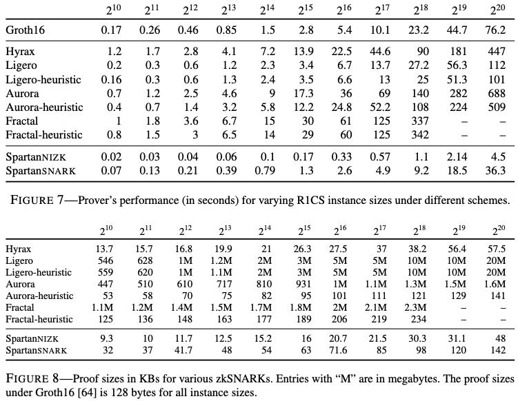
According to the table below, which is taken from the paper, among the proof-succinct NIZKs, SpartanNIZK is 100× faster than Hyrax, 113× faster than Aurora, and 22× faster than Ligero at $$2^{20}$$ constraints. The commitment scheme used for this benchmark is Hyrax-PC over curve25519 ([ref](https://youtu.be/DyK86YMj7XU?t=1427)).
Performance benchmark
## References
* #### [Spartan: Efficient and general-purpose zkSNARKs without trusted setup](https://eprint.iacr.org/2019/550)
> Written by [Batzorig Zorigoo](https://app.gitbook.com/u/cO1lUla01ZW0seepO37jMHFTxg42 "mention") of Fractalyze