# FRI

Short for “Fast Reed-Solomon Interactive Oracle Proofs of Proximity”, the FRI Protocol is a [polynomial commitment scheme](https://docs.scroll.io/en/learn/zero-knowledge/polynomial-commitment-schemes/) designed for zkSTARKS. All Interactive Oracle Proofs of Proximity (IOPPs) are designed to verify that a large dataset or computation closely matches a specific structure using only a few queries. FRI, in particular, addresses the challenge of low-degree testing within this framework. But what is “Low Degree Testing,” you ask? Let’s talk about the “Reed-Solomon” portion in FRI’s title to explain.

## Background

### Reed-Solomon Encoding

We’ll pull from [Risc Zero’s intuitive explanation](https://www.youtube.com/watch?v=Yu9DHhdSqQo\&list=PLcPzhUaCxlCjdhONxEYZ1dgKjZh3ZvPtl\&index=20) and Vitalik’s article “[STARKs, Part II: Thank Goodness It’s FRI-day](https://vitalik.eth.limo/general/2017/11/22/starks_part_2.html)” to explain how Reed-Solomon Encoding works and introduce the idea of “low-degree testing.” Feel free to take an additional look at [STIR](https://fractalyze.gitbook.io/intro/~/revisions/6ILOvDSvW4zAg8fUzupj/zk/stark/stir) to understand more about the technicalities behind Reed-Solomon codes.

The goal of Reed-Solomon encoding is to securely pass a message successfully to another party. Let’s look at an example:

Say User A wants to send the message “ABC” to a User B with Reed-Solomon encoding…

First, User A converts this message into a polynomial of degree "$$\text{total values} - 1$$." In our case, that’s $$\mathsf{len}(ABC) - 1 = 3-1 = 2$$.

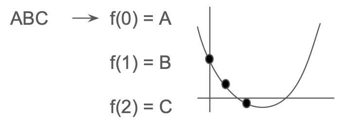
<figure><img src="https://755218234-files.gitbook.io/~/files/v0/b/gitbook-x-prod.appspot.com/o/spaces%2Frwz1ZAZJtK5FHz4Y1esA%2Fuploads%2Fgit-blob-c11e945c0907d906c09ad0856ffab17927251b13%2Fimage.png?alt=media" alt=""><figcaption><p>Figure 1. Reed Solomon Encoding — Converting a message into a polynomial</p></figcaption></figure>

Next, User A evaluates this polynomial on a larger domain of a coset and adds more values to hide the original message.

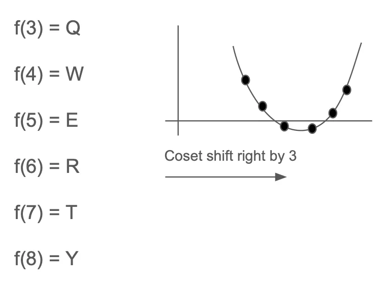
<figure><img src="https://755218234-files.gitbook.io/~/files/v0/b/gitbook-x-prod.appspot.com/o/spaces%2Frwz1ZAZJtK5FHz4Y1esA%2Fuploads%2Fgit-blob-e51bbaadd2dd05c9fea2310757ac1c918383428a%2Fimage.png?alt=media" alt=""><figcaption><p>Figure 2. Reed Solomon Encoding — Extrapolating the polynomial into a larger codeword.</p></figcaption></figure>

This set of evaluations is sent all together to User B and is named the “codeword.”

Let’s say User A was instead a malicious user and attempted to send a faulty codeword instead. We’ll change $$f(3)$$ to $$P$$ instead to illustrate how User B could successfully catch this mistake.

User B first receives the codeword from User A, and tries to check a random value in the codeword, otherwise known as querying. By chance, let’s say, User B tries to check $$f(3)$$. User B uses User A’s codeword values excluding $$f(3) = P$$ to create a Lagrange-based form of a polynomial through interpolation (See[ Barycentric interpolation](https://hackmd.io/@vbuterin/barycentric_evaluation) for more details on interpolation). In our case, this should be a polynomial of degree 2. Using this interpolated polynomial, User B can now calculate the value at $$x=3$$ themselves and find that $$f(3)$$ should equal $$Q$$. Finally, they check this self-calculated value $$f(3) = Q$$ against User A’s previously asserted value of $$f(3) = P$$ and reject the User A’s codeword since the values are not equal.

But what does a rejection actually mean? If we look at figure 2, we can see that if the codeword was valid, all the values should belong to the same line or to the polynomial of the same degree 2. In comparison, in figure 3, we see that one faulty value would jeopardize the degree of the resulting total polynomial by increasing it to a degree higher than 2. This thus introduces the problem of ***low-degree testing***. Low-degree testing tries to ensure a polynomial is of low-degree, which would insinuate that the original polynomial or codeword is valid.

<figure><img src="https://755218234-files.gitbook.io/~/files/v0/b/gitbook-x-prod.appspot.com/o/spaces%2Frwz1ZAZJtK5FHz4Y1esA%2Fuploads%2Fgit-blob-94a110cddc6d819197bc3a2f15ea882382dc174a%2Fimage.png?alt=media" alt=""><figcaption><p>Figure 3. Reed Solomon Encoding — Checking a faulty value in a codeword.</p></figcaption></figure>

### Low-Degree Testing <a href="#id-0ccd" id="id-0ccd"></a>

As you can now see, low-degree testing refers to the process of ensuring a polynomial is of low-degree or smaller than a certain degree. But why is FRI needed specifically for low-degree testing? Well, this ties back to the original goal of IOPPs to use fewer queries or reduce the overall query load. In our example earlier we mentioned that if User B queries a value, a total of $$d+1$$ other values must be needed to interpolate the polynomial at the given value, with d being the degree of the original polynomial. This results in the naive complexity of each query equaling $$O(d+1)$$. However, as an IOPP, The FRI protocol manages to achieve low-degree testing with only $$O(\log(d))$$ queries, as instead of using expensive interpolation, FRI folds the polynomial into a constant to check the degree.

## The FRI Protocol

As Risc Zero explains in their video [“FRI in 2 minutes,”](https://youtu.be/YiYN6UgE8sQ?feature=shared) the FRI protocol is a process in which a polynomial is folded a number of times to reduce the problem size and then verified by a limited number of queries. The FRI protocol is split into two phases: the Commit Phase and the Query Phase. In the commit phase, the prover recursively folds the polynomial and commits their evaluations, while in the query phase, the verifier checks the folded evaluations through their own calculations. Note that while the concept of the FRI protocol mentions folding can by done at any constant scale *k*, we will explain the process of 2-folding for simplicity and for its prevalence in FRI in code.

The naive version of the FRI protocol consists of the implementation outlined below, with a simple difference of making it non-interactive by introducing a separate challenger. To see naive FRI in code, refer to [LambdaClass’s](https://github.com/lambdaclass/lambdaworks/tree/main/provers/stark/src/fri) implementation for Rust or [Kroma’s](https://github.com/kroma-network/tachyon/blob/main/tachyon/crypto/commitments/fri/simple_fri.h) implementation in C++.

### The Input

The input to the protocol is a polynomial $$f\_0(x)$$ linked with a bounding degree by which the polynomial’s degree should be at or less than.

### The Commit Phase

As aforementioned, the commit phase follows the prover folding the polynomial to a digestible size. *Going forward, we’ll refer to example-specific sections with “(EX)”.*

1. With knowledge of the input polynomial $$f\_0(x)$$, the prover evaluates the polynomial on a given domain ($$f\_0({\omega\_0}^0), f\_0({\omega\_0}^1),..., f\_0({\omega\_0}^{n-1})$$, where $$\omega$$ is a [root of unity](https://medium.com/@aiswaryamathur/understanding-fast-fourier-transform-from-scratch-to-solve-polynomial-multiplication-8018d511162f) and n is the domain size). This evaluation is usually done with [FFT](https://medium.com/@aiswaryamathur/understanding-fast-fourier-transform-from-scratch-to-solve-polynomial-multiplication-8018d511162f) (Fast-Fourier Transformation). These evaluations all together act as a single Reed-Solomon codeword as if a single evaluation is wrong and is caught, the polynomial is guaranteed to be of high-degree.
   1. (*EX) The prover calculates* $$f\_0({\omega\_0}^0)=A, f\_0({\omega\_0}^1)=B,f\_0({\omega\_0}^2)=C,f\_0({\omega\_0}^3)=D$$
2. These evaluations are then used to create the leaves of a [Merkle tree](https://medium.com/coinmonks/merkle-tree-a-simple-explanation-and-implementation-48903442bc08), and the resulting Merkle root is committed to the verifier \[MT root]. These evaluations can also be interpreted as the Reed Solomon codeword of the FRI protocol.

   1. (*EX) The prover creates a Merkle tree from* $$A, B, C, D$$ *and commits the root* $$R$$:

   <figure><img src="https://755218234-files.gitbook.io/~/files/v0/b/gitbook-x-prod.appspot.com/o/spaces%2Frwz1ZAZJtK5FHz4Y1esA%2Fuploads%2Fgit-blob-e906b6830a15c44b5d883980229a90528a8a64b4%2Fimage.png?alt=media" alt=""><figcaption><p>Figure 4. Resulting Merkle Tree from the example evaluations of the original polynomial</p></figcaption></figure>
3. After receiving the Merkle Root, the verifier replies with a challenge $$\beta$$ in response.
4. With this $$\beta$$, the prover calculates the folded polynomial. Let’s look at how this works:

First, $$f\_0(x)$$ is split into two different parts: the terms with a degree of an even number and the terms with a degree of an odd number.

$$
f\_o(x) = f\_{0\_\mathsf{even}}(x^2) + X \cdot f\_{0\_\mathsf{odd}}(x^2)
$$

Then the folded polynomial is created from these two parts along with the challenge:

$$
f\_1(x) = f\_{0\_\mathsf{even}}(x)+\beta\_0\cdot f\_{0\_\mathsf{odd}}(x)
$$

Let’s check how this works with an example:

$$
f\_{0}(x)=x^4+5x^3+9x^2+8x+7
$$

Our even and odd degree terms would then be split up as such:

$$
f\_{0\_\mathsf{even}}(x^2) = x^4+5x^2+7\f\_{0\_\mathsf{even}}(x)=x^2+9x+7\ \ \x\cdot f\_{0\_\mathsf{odd}}(x^2)=5x^3+8x\f\_{0\_\mathsf{odd}}(x)=5x+8
$$

From these two split polynomials we can now create our folded polynomial:

$$
f\_1(x)=(x^2+9x+7)+\beta\_0\cdot (5x+8)\f\_1(x)=x^2+(9+5\beta\_0)x+(7+8\beta\_0)
$$

Finally, we can see that our polynomial $$f\_0(x)$$ of degree 4 has been successfully folded in half to polynomial $$f\_1(x)$$ of degree 2. Thus all polynomials of degree $$d$$ will be folded to a polynomial of degree $$\lfloor d/2 \rfloor$$.

5. Next, the prover is evaluated on the given sub-domain. Note that the domain size is reduced by half every fold, resulting in $${\omega\_0}^0 ={\omega\_1}^0$$ and $${\omega\_0}^2={\omega\_1}^1$$. In other words, $${\omega\_i}^{2n}={\omega\_{i+1}}^n$$.
   1. (*EX) Let’s say our folded polynomial had the following evaluations* $$f\_1({\omega\_1}^0)=N$$ *and* $$f\_1({\omega\_1}^1) =O$$*.*
6. Finally, the evaluations are used to create a Merkle tree, and the root of the resulting Merkle tree is committed.
   1. (*EX) The prover creates a Merkle tree from* $$N$$ *and* $$O$$ *and commits the root* $$R$$*:*

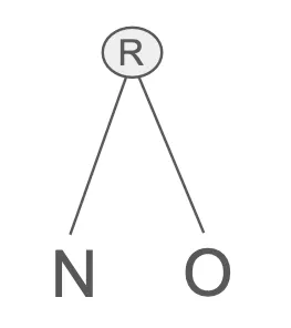
      <figure><img src="https://755218234-files.gitbook.io/~/files/v0/b/gitbook-x-prod.appspot.com/o/spaces%2Frwz1ZAZJtK5FHz4Y1esA%2Fuploads%2Fgit-blob-5e83cb3eb4d500f04ca1de7217d621467eadfcd0%2Fimage.png?alt=media" alt=""><figcaption><p>Figure 5: Resulting Merkle Tree from the example’s first folded polynomial evaluations</p></figcaption></figure>
7. This recursive folding process continues until the polynomial is reduced to a constant and committed as the final result. Note that the evaluations of the polynomials are seen as the codewords within Reed-Solomon encoding, hence, the title of FRI.
   1. (*EX) The prover folds the polynomial one more time and gets* $$f\_2({\omega\_2}^0)=T$$ *and commits* $$T$$*.*

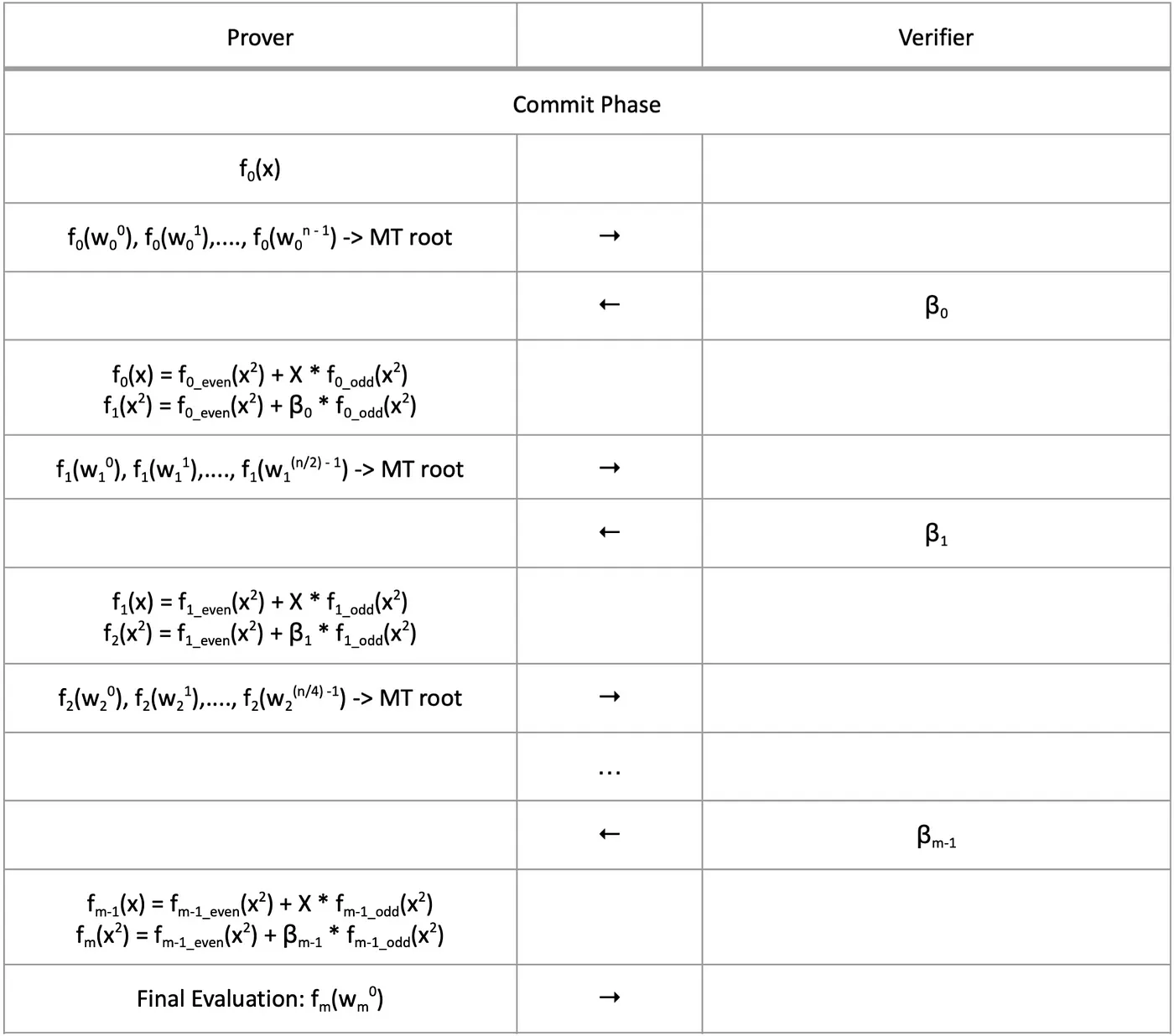
<figure><img src="https://755218234-files.gitbook.io/~/files/v0/b/gitbook-x-prod.appspot.com/o/spaces%2Frwz1ZAZJtK5FHz4Y1esA%2Fuploads%2Fgit-blob-02df03ef879046c47d1c5c3e61174f847655c559%2Fimage.png?alt=media" alt=""><figcaption><p>Figure 6. The Commit Phase of the FRI protocol illustrated in a table, where n = domain size and m = the total number of folding rounds aka ⌈log(d)⌉ with d being the maximum degree</p></figcaption></figure>

### The Query Phase

In the query phase, the verifier ensures that the prover’s polynomial evaluations are valid through queries. The following explanations describe the process of running a single query.

1. The verifier queries a random challenge $$x$$ to the prover.
2. The prover sends $$f\_i(x),f\_i(-x)$$ where $$i$$ starts at $$0$$ and the individual Merkle tree proof for each evaluation back to the verifier.
3. The verifier verifies the Merkle tree proofs.
4. The verifier uses $$f\_i(x)$$ and $$f\_i(-x)$$ to create $$f\_{i+1}(x^2)$$ themselves and checks with the prover’s given answer. How does the verifier do this? Let’s take a look:

$$
f\_i(x) = f\_{i\_\mathsf{even}}(x^2)+X\cdot f\_{i\_\mathsf{odd}}(x^2)\f\_i(-x) = f\_{i\_\mathsf{even}}(x^2)-X\cdot f\_{i\_\mathsf{odd}}(x^2)
$$

Through solving the system of equations of $$f\_i(x)$$ and $$f\_i(-x)$$, we can get $$f\_{i\_ even}(x^2)$$ and $$f\_{i\_odd}(x^2)$$.

$$
f\_{i\_\mathsf{even}}(x^2)= \frac{f\_i(x) + f\_i(-x)}{2}\f\_{i\_\mathsf{odd}}(x^2)= \frac{f\_i(x) - f\_i(-x)}{2x}
$$

Finally, with $$f\_{i\_ even}(x^2)$$ and $$f\_{i\_ odd}(x^2)$$ , we can create $$f\_{i+1}(x^2)$$ or the next folded polynomial’s evaluations.

$$
f\_{i+1}(x^2) = f\_{i\_\mathsf{even}}(x^2)+\beta\_i\cdot f\_{i\_\mathsf{odd}}(x^2)\ \ \\\begin{align\*}f\_{i+1}(x^2) &=\frac{f\_i(x)+f\_i(-x)}{2}+\beta\_i\cdot\frac{f\_i(x)-f\_i(-x)}{2x}\ &=\frac{xf\_i(x)+xf\_i(-x)+\beta\_if\_i(x)-\beta\_if\_i(-x)}{2x}\\&=\frac{(x+\beta\_i)f\_i(x)+(x-\beta\_i)f\_i(-x)}{2x}\\&=\frac{(1+\beta\_ix^{-1})f\_i(x)+(1-\beta\_ix^{-1})f\_i(-x)}{2}\end{align\*}
$$

Thus with the received $$f\_i(x)$$ and $$f\_i(-x)$$ and knowing $$x$$ and $$\beta\_i$$, the verifier can create $$f\_{i+1}(x^2)$$.

5. The prover continues to send the $$f\_i(x)$$ and $$f\_i(-x)$$evaluations incrementing $$i$$ by $$1$$ each round, while the verifier continues calculating and verifying until the final evaluation is verified (i.e. recursively run steps 2-4).
6. This query process is repeated to the desired amount of queries.

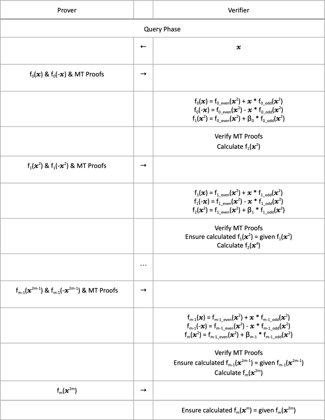
<figure><img src="https://755218234-files.gitbook.io/~/files/v0/b/gitbook-x-prod.appspot.com/o/spaces%2Frwz1ZAZJtK5FHz4Y1esA%2Fuploads%2Fgit-blob-445b537038a4a2afc07965adb4c5f683d484dfb0%2Fimage.png?alt=media" alt=""><figcaption><p>Figure 7. A single query of the Query Phase illustrated in a table, where n = domain size and m = the total number of folding rounds aka ⌈log(d)⌉ with d being the maximum degree</p></figcaption></figure>

## **Conclusion** <a href="#f3df" id="f3df"></a>

The FRI Protocol stands as a valuable IOPP protocol to reduce the number of queries in the case of low-degree testing. While the general scheme simply involves recursively folding a polynomial, the [numerous advances in adding security and optimizations](https://fractalyze.gitbook.io/intro/~/revisions/6ILOvDSvW4zAg8fUzupj/zk/stark/fri/fri-security-features-and-optimizations) additionally complicates the protocol. If you choose to dive more into the FRI protocol, I recommend you look at the following references for more information.

## **References** <a href="#eb26" id="eb26"></a>

* [**Reed-Solomon Codes**](https://youtu.be/Yu9DHhdSqQo?feature=shared) by the Risc Zero Study Club — A good intro to RS Codes
* [**Intro to FRI**](https://youtu.be/j35yz22OVGE?feature=shared) by the Risc Zero Study Club — A good intro to FRI
* [**FRI Mechanics**](https://youtu.be/wqRuoyH3Mqk?feature=shared) by the Risc Zero Study Club — A good view into the process of FRI
* [**Low Degree Testing: The Secret Sauce of Succinctness**](https://medium.com/starkware/low-degree-testing-f7614f5172db) by [StarkWare](https://medium.com/u/373f5878a0c6?source=post_page---user_mention--85e979ee39fc--------------------------------)— A good starter overview on FRI
* [**STARKs, Part II: Thank Goodness It’s FRI-day**](https://vitalik.eth.limo/general/2017/11/22/starks_part_2.html) by Vitalik Buterin — Provides insight to the concept behind FRI
* [**A Diagram of the FRI Protocol**](https://x.com/EllipticHector/status/1639698732064165893) by Elliptic Hector — A good visual of the FRI Protocol
* [**Fast Reed-Solomon IOP (FRI) Proximity Test**](https://rot256.dev/post/fri/) — A good hands-on example of FRI
* [**How to code FRI from scratch**](https://blog.lambdaclass.com/how-to-code-fri-from-scratch/) by LambdaClass — Provides a code and computation viewpoint of FRI
* [**Anatomy of a STARK, Part 3: FRI**](https://aszepieniec.github.io/stark-anatomy/fri.html) — An extensive dive into FRI
* [**Fast Reed-Solomon Interactive Oracle Proofs of Proximity**](https://eccc.weizmann.ac.il/report/2017/134/) — The original FRI paper
* [**ethSTARK Documentation — Version 1.2**](https://eprint.iacr.org/2021/582.pdf) by the StarkWare Team — Provides some valuable sections outlining security features and optimizations to add to FRI
* [**RedShift: Transparent SNARKs from List Polynomial Commitments**](https://eprint.iacr.org/2019/1400.pdf) by Matter Labs — Section 8 and Section F provide an in-depth view of added security features and optimizations
* [**A summary on the FRI low degree test**](https://eprint.iacr.org/2022/1216.pdf) by Polygon Labs — An extensive view into Two Adic FRI

> Written by [Ashley Jeong](https://app.gitbook.com/u/PNJ4Qqiz7kSxSs58UIaauk95AO43 "mention") of Fractalyze