# cuZK

## Introduction

Modern GPUs are equipped with thousands of cores, offering immense parallel computing power. This naturally raises the question: **can we fully exploit this parallelism to accelerate cryptographic protocols like zkSNARKs?** In particular, **Multi-Scalar Multiplication (MSM)**—a core bottleneck in zkSNARK provers—appears to be a promising target for GPU acceleration.

However, existing MSM algorithms are often optimized for CPU execution and assume **uniformly distributed scalars**, which leads to **load imbalance** and **inefficient GPU utilization** in real-world scenarios where scalar distributions are highly non-uniform or clustered.

**cuZK** addresses this gap. It is a high-performance computation framework specifically designed for **GPU-based zkSNARK systems**, with the goal of maximizing the throughput of MSM.

## Background

### Sparse Matrix Storage Format

While there are other formats such as [COO](https://en.wikipedia.org/wiki/Sparse_matrix#Coordinate_list_\(COO\)) and [CSC](https://en.wikipedia.org/wiki/Sparse_matrix#Compressed_sparse_column_\(CSC_or_CCS\)), this section introduces only the **ELL** and **CSR** formats, as they are used in the paper.

<figure><img src="https://755218234-files.gitbook.io/~/files/v0/b/gitbook-x-prod.appspot.com/o/spaces%2Frwz1ZAZJtK5FHz4Y1esA%2Fuploads%2FiWpCz2be2iOSb2hUEQw0%2Fimage.png?alt=media&#x26;token=477f075a-77d8-4976-b231-62c026ce1704" alt=""><figcaption></figcaption></figure>

#### ELL (ELLPACK)

**ELL** stores a fixed number of non-zero elements **per row**. Its highly regular structure makes it **well-suited for GPU computation**.

**Structure**

ELL consists of two 2D arrays and one 1D array:

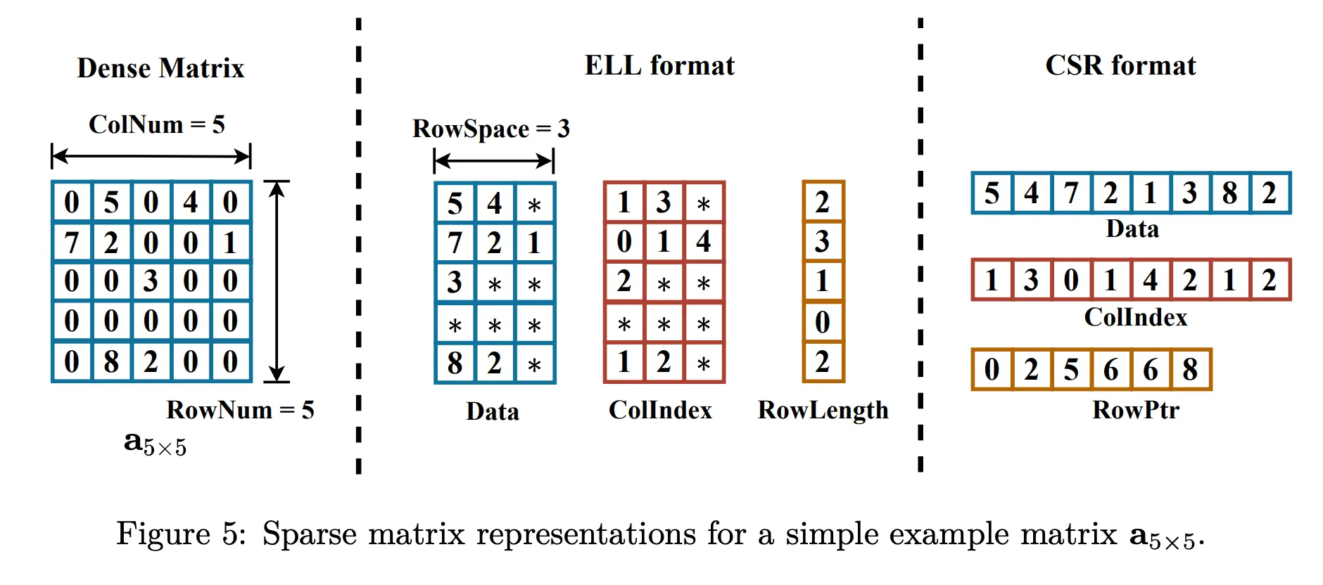
<table><thead><tr><th width="282.903564453125">Array</th><th>Description</th></tr></thead><tbody><tr><td><code>values</code></td><td>Non-zero values in each row; padded with zeros if needed</td></tr><tr><td><code>col_indices</code></td><td>Column indices of the values; dummy indices used for padding</td></tr><tr><td><code>row_length</code></td><td>Actual number of non-zero elements in each row</td></tr></tbody></table>

→ **All rows are padded to have the same number of elements.**

**Example**

Given matrix:

$$
\begin{bmatrix}
10 & 0 & 20 & 0 \\
0 & 0 & 30 & 0 \\
0 & 0 & 0 & 40
\end{bmatrix}
$$

ELL representation:

* `values` = $$\begin{bmatrix}  10 & 20 \ 30 & 0 \ 40 & 0 \end{bmatrix}$$
* `col_indices` = $$\begin{bmatrix}  0 & 2 \ 2 & -1 \ 3 & -1 \end{bmatrix}$$
* `row_length` = $$(2, 1, 1)$$

**Pros**

* Regular memory layout → **GPU-optimized** (predictable access patterns)

**Cons**

* If the number of non-zero elements varies across rows, **excessive padding** leads to **wasted memory**
* Not suitable for dynamic or highly irregular matrices due to padding overhead

#### CSR (Compressed Sparse Row)

**CSR** is a widely used format that **compresses sparse matrices row-wise**. It is memory-efficient and versatile for computation.

**Structure**

CSR consists of three 1D arrays:

| Array         | Description                             |
| ------------- | --------------------------------------- |
| `values`      | Non-zero values of the matrix           |
| `col_indices` | Column indices for each value           |
| `row_ptr`     | Index in `values` where each row starts |

**Example**

Given matrix:

$$
\begin{bmatrix}
10 & 0 & 20 & 0 \\
0 & 0 & 30 & 0 \\
0 & 0 & 0 & 40
\end{bmatrix}
$$

CSR representation:

* `values` = $$(10, 20, 30, 40)$$
* `col_indices` = $$(0, 2, 2, 3)$$
* `row_ptr` = $$(0, 2, 3, 4)$$

***

#### Pros

* **Memory-efficient** representation
* Optimized for **row-wise operations**, such as matrix-vector multiplication

#### Cons

* Varying row lengths may cause **imbalanced memory access patterns**

## Protocol Explanation

### Notations

* $$n$$: The number of points
* $$\lambda$$: The bit-width for scalar field
* $$s$$: The bit-width for each window
* $$t$$: The number of threads

### Naive Approaches

While Pippenger’s algorithm is originally optimized for large-scale MSM, several parallelization strategies are explored to adapt it to **GPU environments**. Below are three naive partitioning approaches along with a complexity analysis for each.

> 📌 Note: The computational complexity here slightly differs from what is presented in the paper.

#### Approach 1: **Window-Level Parallelism**

**Core Idea**

* Decompose Pippenger into $$\left\lceil \frac{\lambda}{s} \right\rceil$$ parts.
* Each thread computes one window $$W\_j$$.
* The full MSM is restructured as:

$$
Q = \sum\_{i=1}^{n} k\_i P\_i  = \sum\_{j=1}^{\left\lceil\frac{\lambda}{s}\right\rceil} 2^{(j-1)s} W\_j
$$

**Advantages**

* Preserves the structure of **Pippenger’s algorithm**

**Disadvantages**

* The number of windows $$\left\lceil \frac{\lambda}{s} \right\rceil$$ is relatively small (e.g., $$\lambda = 256$$, $$s = 16$$ → only 16 windows), however modern GPUs have thousands of threads → **low parallelism**

**Computational Complexity (per thread)**

$$
\lambda \times \mathsf{PointDouble} + (n + 2^{s+1} + \left\lceil \frac{\lambda}{s}\right\rceil)\times \mathsf{PointAdd}
$$

* $$n \times \mathsf{PointAdd}$$: Bucket accumulation
* $$2^{s+1} \times \mathsf{PointAdd}$$: Bucket reduction
* $$\lambda \times \mathsf{PointDouble} + \left\lceil \frac{\lambda}{s}\right\rceil \times \mathsf{PointAdd}$$: Window reduction

#### Approach 2: **Thread-Level MSM Partitioning**

**Core Idea**

* Decompose MSM computation into $$t$$ parts.
* Each thread performs serial Pippenger $$\sum\_{\ell = (j-1)\frac{n}{t} +1}^{j \frac{n}{t}} k\_{\ell} P\_{\ell}$$.
* The full MSM is restructured as:

$$
Q = \sum\_{i=1}^{n} k\_i P\_i  = \sum\_{j=1}^{t} \left( \sum\_{\ell = (j-1)\frac{n}{t} +1}^{j \frac{n}{t}} k\_{\ell} P\_{\ell} \right)
$$

**Advantages**

* Scales easily with the number of threads → **good GPU resource utilization**

**Disadvantages**

* Each thread handles fewer data points, which **weakens the bucket accumulation benefit of Pippenger**

**Computational Complexity (per thread)**

$$
\lambda \times \mathsf{PointDouble} + \left(\left\lceil\frac{\lambda}{s}\right\rceil\left(\frac{n}{t} + 2^{s+1}\right) + \log t\right)\times \mathsf{PointAdd}
$$

* $$\left\lceil \frac{\lambda}{s}\right\rceil \frac{n}{t}  \times \mathsf{PointAdd}$$: Bucket accumulation
* $$\left\lceil \frac{\lambda}{s}\right\rceil 2^{s+1}  \times \mathsf{PointAdd}$$: Bucket accumulation
* $$\lambda \times \mathsf{PointDouble}$$: Window reduction (Shouldn't it be $$\lambda \times \mathsf{PointDouble} + \left\lceil \frac{\lambda}{s}\right\rceil \times \mathsf{PointAdd}$$?  :thinking:)
* $$\log t \times \mathsf{PointAdd}$$: Final Window reduction

Let $$T(t)$$ be the time complexity for summing $$t$$ values in parallel:

$$
T(t) = \log\_2 t
$$

```
Level 0: P1   P2   P3   P4   P5   P6   P7   P8
           \  /     \  /     \  /     \  /
Level 1:    A1       A2       A3       A4
                \     /         \     /
Level 2:         B1               B2
                      \         /
Level 3:               Final Result

```

#### Approach 3: **Hybrid Parallelism (Approach 1 + 2)**

**Core Idea**

* Decompose MSM computation into $$\frac{t}{\left\lceil \frac{\lambda}{s}\right\rceil}$$ parts.
* Each thread computes one window $$W\_{\ell, j}$$.
* The full MSM is restructured as:

$$
Q = \sum\_{i=1}^{n} k\_i P\_i  = \sum\_{\ell=1}^{\frac{t}{\left\lceil \frac{\lambda}{s}\right\rceil}} \left( \sum\_{j = 1}^{\left\lceil \frac{\lambda}{s}\right\rceil} 2^{(j-1)s} W\_{\ell, j}\ \right)
$$

Let $$W\_{\ell, j}$$​ denote the **partial sum of the** $$j$$**-th window** computed from the $$\ell$$-th MSM partition. Specifically,

$$
W\_{\ell, j} = \sum\_{i \in \mathcal{I}*\ell} m*{ij}
$$

where:

* $$\mathcal{I}\_\ell$$​ is the index set of base points and scalars assigned to the $$\ell$$-th thread partition
* $$m\_{ij}$$​ is the $$j$$-th $$s$$-bit chunk of scalar $$k\_i$$

**Advantages**

* Combines **Pippenger’s structure** with **GPU-level parallelism**
* Enables use of **all available GPU threads** → achieves **high parallelism**

**Disadvantages**

* Each thread handles fewer data points, which **weakens the bucket accumulation benefit of Pippenger.** (But it's better than Approach 2)
* Cannot achieve **perfect linear speedup** (i.e., where parallel execution speed improves proportionally with the number of threads). In particular, the number of buckets $$2^{s+1}$$ are not divisible by the number of threads.

**Computational Complexity (per thread)**

$$
\lambda \times \mathsf{PointDouble} + \left(\left\lceil\frac{\lambda}{s}\right\rceil\left(\frac{n}{t} + 1 \right) + 2^{s+1} + \log (t / \left\lceil \lambda /s \right\rceil)\right)\times \mathsf{PointAdd}
$$

* $$\left\lceil \frac{\lambda}{s}\right\rceil \frac{n}{t}  \times \mathsf{PointAdd}$$: Bucket accumulation
* $$2^{s+1} \times \mathsf{PointAdd}$$: Bucket reduction
* $$\lambda \times \mathsf{PointDouble} + \left\lceil \frac{\lambda}{s}\right\rceil \times \mathsf{PointAdd}$$: Window reduction
* $$\log (t / \left\lceil \lambda /s \right\rceil) \times \mathsf{PointAdd}$$: Final Window reduction

### Overview

**cuZK** designs a pipeline that **fully leverages the bucket structure of the Pippenger algorithm** to perform **high-throughput large-scale MSM computation on GPUs**. The overall workflow is outlined below.

<figure><img src="https://755218234-files.gitbook.io/~/files/v0/b/gitbook-x-prod.appspot.com/o/spaces%2Frwz1ZAZJtK5FHz4Y1esA%2Fuploads%2FEJdMq1vNht1WDhF6RCXQ%2Fimage.png?alt=media&#x26;token=b3939e5e-caa3-4a7b-b7b3-be543f7f0f8e" alt=""><figcaption></figcaption></figure>

#### Step 1: Store All Base Points $$P\_i$$ in an ELL Sparse Matrix

An empty sparse matrix of size $$t \times (2^s - 1)$$ is created in **ELL format**, which is chosen for its suitability for **parallel processing**.

**Example (**$$n = 8$$**,** $$s = 3$$, $$t = 4$$**):**

$$
\begin{align\*}
G&=4P\_1 + 0P\_2 + 7P\_3 + 3P\_4 + 0P\_5

* 3P\_6 + 4P\_7 + 3P\_8 \\
  &= 4P\_1 + 7P\_3 + 3P\_4 + 3P\_6 + 4P\_7 + 3P\_8 \\
  &=(4P\_1) + (3P\_6) + (7P\_3 + 4P\_7) + (3\underbrace{(P\_4 +P\_8)}\_{P\_s})
  \end{align\*}
  $$

- Base points with zero scalars are omitted.
- Points like $$P\_4 + P\_8$$ are accumulated and stored as a **bucket point** ($$P\_s$$).

**ELL format:**

$$
M = \begin{bmatrix}
0 & 0 & 0 & 0 & P\_1 & 0 & 0 & 0 \\
0 & 0 & 0 & P\_6 & 0 & 0 & 0 & 0 \\
0 & 0 & 0 & 0 & P\_7 & 0 & 0 & P\_3 \\
0 & 0 & 0 & P\_s & 0 & 0 & 0 & 0 \\
\end{bmatrix}
$$

* `values` = $$\begin{bmatrix}  P\_1 & 0 \ P\_6 & 0 \ P\_3 & P\_7 \ P\_s & 0 \end{bmatrix}$$
* `col_indices` = $$\begin{bmatrix}  4 & -1 \ 3 & -1 \ 7 & 4 \  3 & -1 \end{bmatrix}$$
* `row_length` = $$(1, 1, 2, 1)$$

**Optimizations**

* Points are stored in **global memory** via **indices or pointers**, so all threads can access them.
* To avoid the latency of naive memory transfers, [**multi-streaming** is used to **overlap CPU-GPU data transfer and computation**](#overlapping-data-transfer-with-multi-streaming).
* Assuming complexity from $$\mathsf{PointAdd}$$ and $$\mathsf{PointDouble}$$, optimal $$s$$ is chosen for fixed $$\lambda$$, $$n$$, and $$t$$.\
  → For example, with $$\lambda = 255$$, $$n = 2^{20}$$, and $$t = 5120$$ (V100 GPU), $$s = 16$$ was found to be optimal.

#### Step 2: Convert the Sparse Matrix from ELL to CSR

**Why convert?**

1. ELL format introduces **zero padding**, making it memory-inefficient.
2. CSR is better suited for **matrix-vector multiplication** and has **well-established algorithms** for efficient computation.

**CSR format:**

* `values` = $$(P\_1, P\_6, P\_3, P\_7, P\_s)$$
* `col_indices` = $$(4, 3, 7, 4, 3)$$
* `row_ptr` = $$(0, 1, 2, 4, 5)$$

#### Step 3: Transpose the CSR Matrix

**Implemetations:**

Performed using a **RadixSort-based scheme**:

1. **Extract Row Indices**:

* Use CSR `row_ptr` to compute row positions
* Store in `RowIndex`

| Index | Value    | ColIndex | RowIndex |
| ----- | -------- | -------- | -------- |
| 0     | $$P\_1$$ | 4        | 0        |
| 1     | $$P\_6$$ | 3        | 1        |
| 2     | $$P\_3$$ | 7        | 2        |
| 3     | $$P\_7$$ | 4        | 2        |
| 4     | $$P\_s$$ | 3        | 3        |

2. **Triplet Formation & Sorting**:

* Create triplets: `<ColIndex, Data, RowIndex>`
* Sort using `ColIndex` as key
* Sorted outputs:
  * `Data` → becomes transposed matrix `Data`
  * `RowIndex` → becomes transposed `ColIndex`

| Index | Before Sort      | After Sort       |
| ----- | ---------------- | ---------------- |
| 0     | $$(4, P\_1, 0)$$ | $$(3, P\_6, 1)$$ |
| 1     | $$(3, P\_6, 1)$$ | $$(3, P\_s, 3)$$ |
| 2     | $$(7, P\_3, 2)$$ | $$(4, P\_1, 0)$$ |
| 3     | $$(4, P\_7, 2)$$ | $$(4, P\_7, 2)$$ |
| 4     | $$(3, P\_s, 3)$$ | $$(7, P\_3, 2)$$ |

3. **Generate Transposed `row_ptr`**:

* Count the occurrences of the `ColIndex` and compute the [**prefix sum**](https://en.wikipedia.org/wiki/Prefix_sum)&#x20;

| ColIndex | Count |
| -------- | ----- |
| 0        | 0     |
| 1        | 0     |
| 2        | 0     |
| 3        | 2     |
| 4        | 2     |
| 5        | 0     |
| 6        | 0     |
| 7        | 1     |

⇒ `prefix_sum([0, 0, 0, 2, 2, 0, 0, 1]) = [0, 0, 0, 0, 2, 4, 4, 4, 5])`

**Resulting Transposed CSR format:**

The matrix is transposed to **group points by bucket index**:

$$
M^{\mathsf{T}} = \begin{bmatrix}
0 & 0 & 0 & 0 \\
0 & 0 & 0 & 0 \\
0 & 0 & 0 & 0 \\
0 & P\_6 & 0 & P\_s \\
P\_1 & 0 & P\_7 & 0 \\
0 & 0 & 0 & 0 \\
0 & 0 & 0 & 0 \\
0 & 0 & P\_3 & 0 \\
\end{bmatrix}
$$

* `values` = $$(P\_6, P\_s, P\_1, P\_7, P\_3)$$
* `col_indices` = $$(1, 3, 0, 2, 2)$$
* `row_ptr` = $$(0, 0, 0, 0, 2, 4, 4, 4, 5)$$

#### Step 4: SPMV (Sparse Matrix-Vector Multiplication)

Perform multiplication:

$$
M^{\mathsf{T}} \cdot
\begin{bmatrix}
1 \\
1 \\
1 \\
1
\end{bmatrix} = \begin{bmatrix}
0 & 0 & 0 & 0 \\
0 & 0 & 0 & 0 \\
0 & 0 & 0 & 0 \\
0 & P\_6 & 0 & P\_s \\
P\_1 & 0 & P\_7 & 0 \\
0 & 0 & 0 & 0 \\
0 & 0 & 0 & 0 \\
0 & 0 & P\_3 & 0 \\
\end{bmatrix} \cdot
\begin{bmatrix}
1 \\
1 \\
1 \\
1
\end{bmatrix}
=============

\begin{bmatrix}
0 \\
0 \\
0 \\
P\_6 + P\_s \\
P\_1 + P\_7 \\
0 \\
0 \\
P\_3
\end{bmatrix}
=============

\begin{bmatrix}
B\_0 \\
B\_1 \\
B\_2 \\
B\_3 \\
B\_4 \\
B\_5 \\
B\_6 \\
B\_7 \\
\end{bmatrix}
$$

Where each $$B\_\ell$$ is a **bucket sum**.

**Optimizations**

To handle **thread load imbalance** (due to varying row lengths), cuZK introduces **CSR-Balanced**:

<table><thead><tr><th width="211.5665283203125">Step</th><th>Description</th></tr></thead><tbody><tr><td>① Sort rows</td><td>By row length (ascending)</td></tr><tr><td>② Group rows</td><td>Rows are grouped so that <strong>each group has a similar workload</strong>, ensuring balanced warp-level execution.</td></tr><tr><td>③ <a href="https://en.wikipedia.org/wiki/Thread_block_(CUDA_programming)#Warps">Warp</a> scheduling</td><td>One warp handles one group (ensures uniform workload)</td></tr><tr><td>④ Warp allocation</td><td>Warp count is proportional to the number of non-zeros in each group</td></tr></tbody></table>

> ✅ Ensures **balanced thread workloads** → maximizes GPU efficiency

For **scalar SPMV**, the sorting overhead outweighs the benefits. But in our case it's negligible compared to EC point operations so we can safely adopt **CSR-Balanced**.

#### Step 5: Reduce Bucket Points

Decompose bucket reduction into $$t$$ parts:

$$
W\_j = \sum\_{\ell = 1}^{2^s - 1}\ell B\_{\ell, j} = \sum\_{i = 1}^{t} \left( \sum\_{\ell = (i - 1)\frac{(2^s - 1)}{t} + 1}^{\min( i\frac{(2^s - 1)}{t}, 2^s - 1)} \ell B\_{\ell, j} \right)
$$

Use $$t$$ **threads** to perform parallel reduction of $$2^s - 1$$ EC points into a single $$W\_j$$.

For example, if $$s = 3, t = 4$$, this bucket reduction can be computed as follows:

$$
\begin{align\*}
W\_j &= 1B\_{1,j} + 2B\_{2, j} + 3B\_{3, j} + 4B\_{4, j} + B\_{5, j} + 6B\_{6, j} + 7B\_{7, j} \\
&= 1B\_{1,j} + 2B\_{2, j} + 0(B\_{1, j} + B\_{2, j}) + (B\_{3, j} + 2B\_{4, j}) + 2(B\_{3, j} + B\_{4, j}) +  (B\_{5, j} + 2B\_{6, j}) + 4(B\_{5, j} + B\_{6, j}) + B\_{7, j} + 6B\_{7, j} \\
&= \sum\_{i=1}^4 (B\_{2i - 1} + 2B\_{2i}) + 2(i-1)(B\_{2i - 1} + B\_{2i})
\end{align\*}
$$

#### Step 6: Reduce Windows

$$
Q = \sum\_{j = 1}^{\left\lceil \frac{\lambda}{s}\right\rceil} 2^{(s - 1)j} W\_j
$$

#### **Computational Complexity (per thread)**

$$
(\lambda + s) \times \mathsf{PointDouble} + \left(\left\lceil \frac{\lambda}{s} \right\rceil \left( \frac{n}{t} + \frac{2^{s+1}}{t} \right) + s + \log t \right) \mathsf{PointAdd}
$$

* $$\left\lceil \frac{\lambda}{s}\right\rceil \frac{n}{t}  \times \mathsf{PointAdd}$$: Storing points into ELL matrix.
* $$s \times \mathsf{PointDouble} + \left(\left\lceil \frac{\lambda}{s}\right\rceil \left(\frac{2^{s+1}}{t} -1\right) + s + \log t \right) \times \mathsf{PointAdd}$$: SPMV(Bucket Accumulation) + Bucket reduction :thinking:
* $$\lambda \times \mathsf{PointDouble} + \left\lceil \frac{\lambda}{s}\right\rceil \times \mathsf{PointAdd}$$: Window reduction

### MUL Optimization in the Groth Protocol

<figure><img src="https://755218234-files.gitbook.io/~/files/v0/b/gitbook-x-prod.appspot.com/o/spaces%2Frwz1ZAZJtK5FHz4Y1esA%2Fuploads%2FRhnNIJEn3zzuQ9uAxiDS%2Fimage.png?alt=media&#x26;token=e9703dd8-7123-48fa-a8af-58fb308d2dcc" alt=""><figcaption></figcaption></figure>

As shown in the figure above, the [**Groth16**](https://fractalyze.gitbook.io/intro/~/revisions/6ILOvDSvW4zAg8fUzupj/zk/snark/groth16) **protocol** performs a **Matrix-Vector Multiplication (MUL)** operation based on the **R1CS (Rank-1 Constraint System)** matrix generated by compiling the target function (prior to the `INTT` step). This R1CS matrix is typically **very large and sparse**. For example, in Filecoin, **less than 0.1%** of the matrix entries are non-zero. To handle such sparsity efficiently, **sparse matrix optimization techniques** are essential. Accordingly, **cuZK stores the R1CS matrix using the CSR (Compressed Sparse Row) format**.

While many parallel SPMV (Sparse Matrix-Vector Product) techniques exist, **no single scheme performs optimally across all matrix types**.

<table><thead><tr><th width="190.4678955078125">Scheme</th><th>Description</th><th>Limitation</th></tr></thead><tbody><tr><td><strong>CSR-Scalar</strong> [Gar08]</td><td>Each thread handles one row</td><td>Severe <strong>load imbalance</strong> when row lengths vary significantly</td></tr><tr><td><strong>CSR-Vector</strong> [BG09]</td><td>A row is divided across multiple threads</td><td>Only effective in specific scenarios</td></tr><tr><td><strong>CSR-Balanced</strong></td><td>Balances load based on row distribution</td><td>Requires <strong>row sorting</strong>, which increases complexity</td></tr></tbody></table>

Instead of using a fixed static scheme, **cuZK dynamically selects the most suitable SPMV strategy** based on the **statistical characteristics** of the R1CS matrix:

| R1CS Matrix Profile                       | Selected SPMV Scheme |
| ----------------------------------------- | -------------------- |
| **Low variance and low mean row length**  | CSR-Scalar           |
| **Low variance but high mean row length** | CSR-Vector           |
| **High variance in row length**           | CSR-Balanced         |

This adaptive strategy allows cuZK to **avoid performance degradation** by choosing the optimal parallel execution path for the structure of each matrix. While this adaptive strategy incurs overhead—due to sorting and computing statistical properties like mean and variance—this is not an issue because the **R1CS matrix is fixed per circuit** and can be **reused**. As a result, **these computations can be performed offline**, introducing **no runtime overhead** during actual proof generation.

### Full zkSNARK Parallelization on GPU

#### Executing All Operations on the GPU

Even lightweight operations (e.g., variable initialization) are **executed using small GPU kernels**, ensuring that even single-thread tasks run on the GPU. This design **minimizes data movement** between CPU and GPU.

In addition, cuZK integrates with well-known high-speed [**NTT (Number Theoretic Transform)**](https://fractalyze.gitbook.io/intro/~/revisions/6ILOvDSvW4zAg8fUzupj/primitives/number-theoretic-transform) implementations ([GJCC20](https://ieeexplore.ieee.org/document/9201530), [KJPA20](https://arxiv.org/abs/2012.01968), [GXW21](https://ieeexplore.ieee.org/document/9485052)), enabling **complete GPU execution of the entire Groth16 proving pipeline**.

#### Transferring Only Essential Data to the GPU

Only the **three essential storage modules** required for zkSNARK execution are transferred to the GPU:

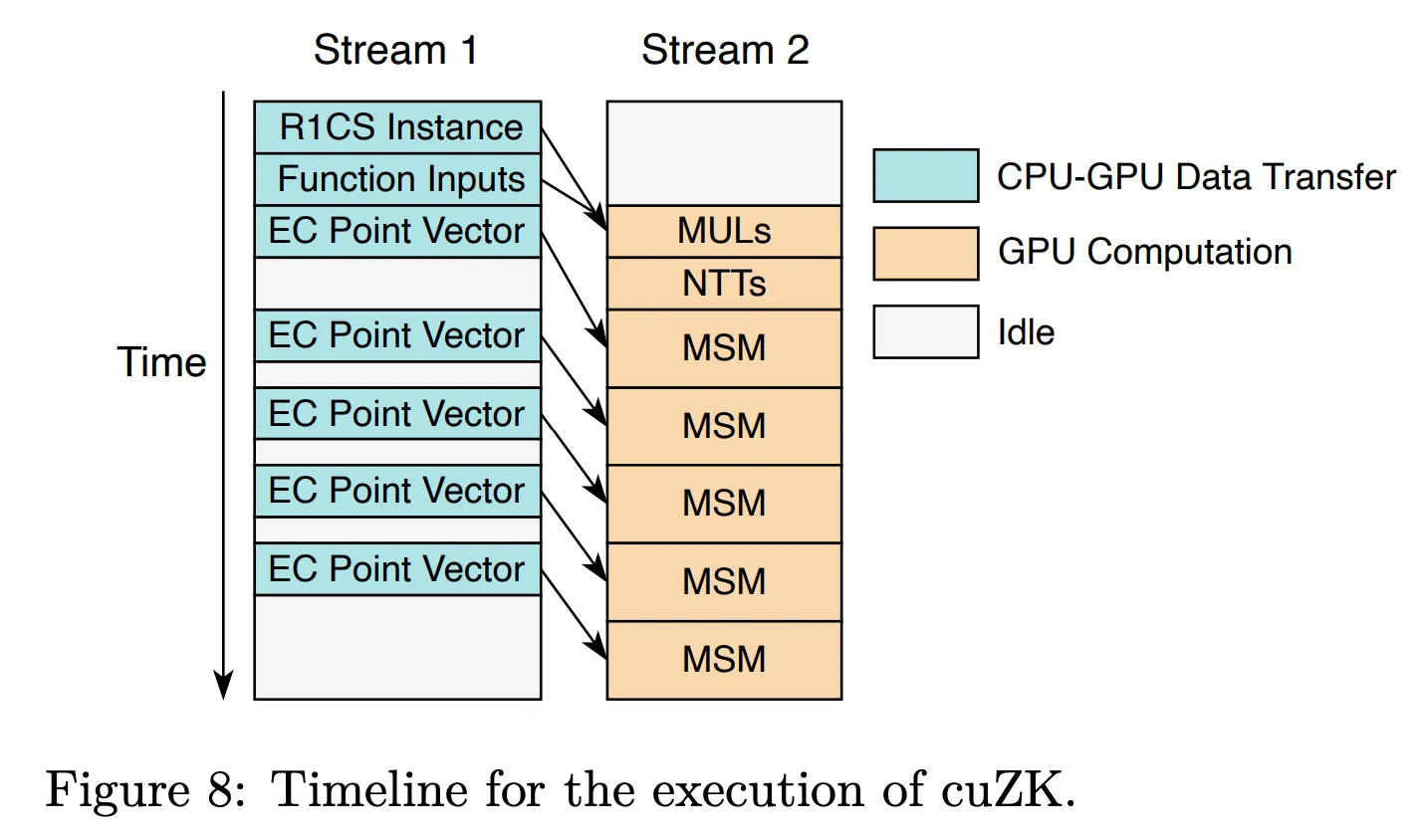
<table><thead><tr><th width="205.943359375">Module</th><th>Description</th></tr></thead><tbody><tr><td>R1CS instance</td><td>Three CSR matrices generated from the circuit</td></tr><tr><td>Function inputs</td><td>Input vector including intermediate computation results</td></tr><tr><td>Prover key</td><td>Large structure composed of elliptic curve (EC) point vectors</td></tr></tbody></table>

Among these, the **R1CS instance and function inputs** are required for the initial **MUL operation**, and must be transferred **before computation begins**.\
The **prover key**, being significantly larger, is transferred **in parallel with computation** using an **overlapping approach**.

#### Overlapping Data Transfer with Multi-Streaming

By leveraging the GPU’s **multi-streaming** capability, **data transfers and computations are overlapped**, thereby removing potential bottlenecks.\
This method **eliminates almost all latency caused by prover key transfers**, and once each MSM computation step is complete, **unused EC point memory is immediately freed**, saving GPU memory.

<figure><img src="https://755218234-files.gitbook.io/~/files/v0/b/gitbook-x-prod.appspot.com/o/spaces%2Frwz1ZAZJtK5FHz4Y1esA%2Fuploads%2Fv7v1l9zwREVu6lTrEinO%2Fimage.png?alt=media&#x26;token=f1288e71-487e-4502-a86b-aac473698593" alt=""><figcaption></figcaption></figure>

## Conclusion

<figure><img src="https://755218234-files.gitbook.io/~/files/v0/b/gitbook-x-prod.appspot.com/o/spaces%2Frwz1ZAZJtK5FHz4Y1esA%2Fuploads%2FcKa5Txe5xWUwZT3ceuC1%2Fimage.png?alt=media&#x26;token=ce2a58b6-8999-4661-8191-7c5ef14e994e" alt=""><figcaption></figcaption></figure>

**Table 1** above shows the experimental setup. The environment uses 8 NVIDIA V100 GPUs connected via **Nvidia** [**NVLink**](https://en.wikipedia.org/wiki/NVLink), which enables **high-speed GPU-to-GPU communication** without routing through the CPU, thereby maximizing parallel processing efficiency.

<figure><img src="https://755218234-files.gitbook.io/~/files/v0/b/gitbook-x-prod.appspot.com/o/spaces%2Frwz1ZAZJtK5FHz4Y1esA%2Fuploads%2Fua0dAQeRSkgp5KyLZOTs%2Fimage.png?alt=media&#x26;token=f139e099-c4cb-40d7-9044-a1b3a20597f8" alt=""><figcaption></figcaption></figure>

**Table 2** presents various baseline MSM implementations used for performance comparisons. Each baseline supports different elliptic curves, and **cuZK was benchmarked against each using the curves supported by the respective implementation**.

<figure><img src="https://755218234-files.gitbook.io/~/files/v0/b/gitbook-x-prod.appspot.com/o/spaces%2Frwz1ZAZJtK5FHz4Y1esA%2Fuploads%2FvIHLF4gne8oSxRzGDLEH%2Fimage.png?alt=media&#x26;token=0e398265-8b5a-4fc6-9630-89230917b47b" alt=""><figcaption></figcaption></figure>

**Table 3** shows MSM performance comparisons on a single GPU across different elliptic curves.\
**cuZK outperforms the previous state-of-the-art (Bellperson)** by **2.08× to 2.29×**.\
In particular, the performance for **Mina** is significantly lower, since it uses a **Straus-based MSM (Refer to** [Bernstein's survey](https://cr.yp.to/papers/pippenger-20020118-retypeset20220327.pdf)), which is **less efficient for large-scale MSM**.

<figure><img src="https://755218234-files.gitbook.io/~/files/v0/b/gitbook-x-prod.appspot.com/o/spaces%2Frwz1ZAZJtK5FHz4Y1esA%2Fuploads%2FRBCqQhxkvMNhS9cWMD8h%2Fimage.png?alt=media&#x26;token=b91da0e2-c40c-4390-85fb-e7647f6ab4db" alt=""><figcaption></figcaption></figure>

As shown in the figure above, the NVIDIA V100 features **5120 CUDA cores**, and cuZK achieves **near-perfect linear speedup** up to the range where $$2^{12} < t < 2^{13}$$.

<figure><img src="https://755218234-files.gitbook.io/~/files/v0/b/gitbook-x-prod.appspot.com/o/spaces%2Frwz1ZAZJtK5FHz4Y1esA%2Fuploads%2FdmIQ1wvgQTnlnpbakofj%2Fimage.png?alt=media&#x26;token=36ad3a3c-8300-4055-b84c-b43b1af7a912" alt=""><figcaption></figcaption></figure>

**Table 4** summarizes multi-GPU MSM performance:

| Size       | 2 × V100 / 1 × V100 | 4 × V100 / 1 × V100 | 8 × V100 / 1 × V100 |
| ---------- | ------------------- | ------------------- | ------------------- |
| $$2^{20}$$ | 1.68                | 3.49                | 6.6                 |
| $$2^{22}$$ | 1.78                | 3.13                | 5.4                 |
| $$2^{24}$$ | 2.1                 | 4.3                 | 7.14                |
| $$2^{26}$$ | 1.92                | 3.77                | 6.55                |

> ⚠️ However, performance **does not scale perfectly linearly** as the number of GPUs increases.
>
> This is due to **imbalanced subtask partitioning**.

***

<figure><img src="https://755218234-files.gitbook.io/~/files/v0/b/gitbook-x-prod.appspot.com/o/spaces%2Frwz1ZAZJtK5FHz4Y1esA%2Fuploads%2FGSUvbaSbUG7qHd2vIiFm%2Fimage.png?alt=media&#x26;token=e3549313-8be7-4b27-9c31-7876b333e6ab" alt=""><figcaption></figcaption></figure>

* For example, if $$\lambda = 255$$ and $$s = 20$$, we have $$\left\lceil \frac{255}{20} \right\rceil = 13$$ windows (subtasks). (See line 17 in the image above)
* With 2 GPUs → assigned 6 and 7 windows respectively → total of 7 block times
* With 4 GPUs → assigned 3, 3, 3, and 4 windows → only 4 block times
* Thus, if the number of subtasks **does not divide evenly** among GPUs, it leads to **load imbalance**, which degrades scalability.

***

<figure><img src="https://755218234-files.gitbook.io/~/files/v0/b/gitbook-x-prod.appspot.com/o/spaces%2Frwz1ZAZJtK5FHz4Y1esA%2Fuploads%2FaBOD1kyxbtKOjjv7t6eS%2Fimage.png?alt=media&#x26;token=949ff7f6-1715-4a7d-9396-a9d57ec95b0c" alt=""><figcaption></figcaption></figure>

**cuZK was also compared against two recent high-performance GPU MSM implementations**:

* [Yrrid](https://github.com/yrrid/submission-msm-gpu)
* [MatterLabs](https://github.com/matter-labs/z-prize-msm-gpu)

While both deliver high performance via **precomputation**, they have limitations:

* Require **large storage space**
* Support **only random scalars** (not optimized for clustered scalars)

<figure><img src="https://755218234-files.gitbook.io/~/files/v0/b/gitbook-x-prod.appspot.com/o/spaces%2Frwz1ZAZJtK5FHz4Y1esA%2Fuploads%2FrP2ubFaA40SrxidaEdvU%2Fimage.png?alt=media&#x26;token=0e50d428-3c98-41dd-b6da-2738bc2fa9d4" alt=""><figcaption></figcaption></figure>

In Groth16 proof generation benchmarks:

* cuZK achieved **up to 2.94× speedup** over Bellperson using **1 V100**
* And **up to 4.86× speedup** using **4 V100s**

Its core contributions are as follows:

1. **A novel sparse matrix-based parallel MSM algorithm**
   * By leveraging the sparse structure of the matrix, cuZK efficiently restructures the MSM computation and mitigates data bottlenecks on GPUs.
2. **Parallelization of MUL (Matrix-Vector Multiplication)**
   * Multiplication operations are parallelized to maximize utilization of GPU cores.
3. **Optimization of CPU-GPU data transfer**
   * Redundant data transfers are eliminated, and
   * Data transfers are overlapped with device-side computation to minimize latency and avoid performance degradation.

🔗 **GitHub (Open Source)**: <https://github.com/speakspeak/cuZK>

## References

* <https://eprint.iacr.org/2022/1321>

> Written by [Ryan Kim](https://app.gitbook.com/u/cPk8gft4tSd0Obi6ARBfoQ16SqG2 "mention") of Fractalyze