# CircleSTARK

## Motivation

There is a trade-off between selecting finite fields that allow for:

1. **Efficient Arithmetic Implementations:** Smaller prime fields, particularly those of special forms like Mersenne primes, enable faster arithmetic operations on standard hardware architectures.
2. **Efficient FFT Support:** Fields need to have smooth multiplicative groups with large two-adic subgroups to support efficient FFTs, which are crucial for STARKs' encoding processes.

One of the most efficient fields for arithmetic seem to be **Mersenne fields**, defined by primes of the form $$p = 2^e − 1$$. In particular, the prime $$p = 2^{31} − 1$$ enables very efficient arithmetic on 32-bit architectures. Since $$2^{32} = 2 \mod{p}$$, a widened product encoded as $$2^{32} \cdot x\_{hi} + x\_{lo}$$ is trivially reduced to a much smaller quantity, $$2 \cdot x\_{hi} + x\_{lo}$$. However, as $$p − 1 = 2 \cdot 3^2 \cdot 7 \cdot 11 \cdot 31 \cdot 151 \cdot 331$$, the multiplicative group lacks two-adic subgroups, which are useful for efficient Cooley-Tukey Fast Fourier Transforms (FFTs).

## Circle Group

For $$p=3\mod{4}$$ , a complex extension field $$\mathbb{F}\_p/(X^2+1)$$ can be defined as:

$$
\mathbb{C}(\mathbb{F}\_p)={x + i\cdot y:x,y\in \mathbb{F}\_p}
$$

For $$p = 1 \mod{4}$$, $$X^2 + 1=0$$ has a solution since by [Legendre Symbol](https://en.wikipedia.org/wiki/Legendre_symbol): $$\frac{-1}{p}=(-1)^{\frac{p-1}{2}}=1$$. This means that $$-1$$ is a [quadratic residue](https://en.wikipedia.org/wiki/Quadratic_residue) and $$X^2+1$$ can be written as $$(X-a)(X+a)$$ making $$\mathbb{F}\_p/(X^2+1)$$ not a field.

The unit circle over $$\mathbb{F}\_p$$ is the algebraic set $$C(\mathbb{F}\_p)={(x,y)\in \mathbb{F}\_p^2 : x^2 + y^2 = 1}$$, or in complex representation:

$$
C(\mathbb{F}\_p)={z\in \mathbb{C}(\mathbb{F}\_p)^\times:z\cdot\bar{z}=1}
$$

where $$\bar{z}$$ denotes the conjugate $$x-iy$$ of $$z=x+iy$$.

**Lemma 1 (Unit circle group).** Let $$\mathbb{F}\_p$$ be a prime field with $$p = 3\mod{4}$$. Then the *unit circle group* $$C(\mathbb{F}\_p)$$ equals the group of $$(p + 1)$$-th roots of unity in $$\mathbb{C}(\mathbb{F}\_p)^\times$$, and has order $$p + 1$$.

Proof: Notice that $$z^p=(x+iy)^p=x^p+(iy)^p=x + (i^p)y=x-iy=\bar{z}$$ so $$x^2+ y^2=z\cdot\bar{z}=z^{p+1}$$. Therefore, $$C(\mathbb{F}\_p)={z\in C(\mathbb{F}\_p)^\times:z^{p+1}=1}$$ which means $$C(\mathbb{F}\_p)$$ is set of all $$(p+1)$$-th roots of unity. Since $$|\mathbb{C}(\mathbb{F}\_p)^\times|=p^2-1$$ is divisible by $$p+1$$, the unit circle group must be the unique subgroup of order $$p + 1$$.

### Group Operations

The $$p + 1$$ points of $$C(\mathbb{F}\_p)$$ form a group with the group operation:

$$
(x\_0, y\_0) \cdot (x\_1, y\_1) := (x\_0 \cdot x\_1 − y\_0 \cdot y\_1, x\_0 \cdot y\_1 + y\_0 \cdot x\_1)
$$

Notice that this equation resembles the $$cos(\alpha + \beta)$$ and $$sin(\alpha+\beta)$$ [formulas](https://mathworld.wolfram.com/TrigonometricAdditionFormulas.html) and is equivalent to rotation over the unit circle.

The group has $$(1, 0)$$ as its identity element, and for any $$P = (P\_x, P\_y) \in C(\mathbb{F}\_p)$$, we shall call

$$
T\_P(x, y) := P \cdot (x, y) = (P\_x \cdot x − P\_y \cdot y, P\_x \cdot y + P\_y \cdot x)
$$

the translation(rotation) by $$P$$.

The squaring map with respect to the group operation is the quadratic map

$$
\pi(x, y) := (x, y) \cdot (x, y) = (x^2 − y^2, 2 \cdot x \cdot y) = (2 · x^2 − 1, 2 \cdot x \cdot y)
$$

and group inverses are given by the degree-one map $$J(x, y) := (x, −y)$$

<figure><img src="https://755218234-files.gitbook.io/~/files/v0/b/gitbook-x-prod.appspot.com/o/spaces%2Frwz1ZAZJtK5FHz4Y1esA%2Fuploads%2Fgit-blob-b68ac0ac09712e89a3365d8c9327206de39176f1%2Fimage.png?alt=media" alt=""><figcaption><p>Figure 1. Blue points under the square operation (left) and inverse operation (right) result in red points.</p></figcaption></figure>

So you can think of $$\pi$$ as doubling the angle it forms with the $$x$$-axis and $$J$$ as a reflection by the $$x$$-axis.

### Twin-coset and Standard Position Coset

First, Figure 2 shows how the subgroups would look like in the circle group.

<figure><img src="https://755218234-files.gitbook.io/~/files/v0/b/gitbook-x-prod.appspot.com/o/spaces%2Frwz1ZAZJtK5FHz4Y1esA%2Fuploads%2Ffsftvuy8kPQC5gktOFua%2Fimage.png?alt=media&#x26;token=5ef5f825-ecc3-453f-bd85-9659860fe94a" alt=""><figcaption><p>Figure 2. Subgroups of size 4, 2, 1 (left to right)</p></figcaption></figure>

Taking a coset of a subgroup means that each point in the subgroup will be rotated by the same amount.

**Definition** Let $$G\_{n-1}$$ be a cyclic subgroup of $$C(\mathbb{F}*p)$$ of size $$|G*{n-1}=2^{n-1}|$$ for $$n\geq1$$. Any disjoint union $$D=Q\cdot G\_{n-1}\cup Q^{-1}\cdot G\_{n-1}$$ with $$Q\cdot G\_{n-1}\cap Q^{-1}\cdot G\_{n-1}=\varnothing$$ is called **twin-coset of size** $$N=2^n$$.

**Remark** Twin-coset maps to itself under inverse, since&#x20;

$$
J(D)=J(Q\cdot G\_{n-1})\cup J(Q^{-1}\cdot G\_{n-1})=Q^{-1}\cdot G\_{n-1}\cup Q\cdot G\_{n-1}
$$

<figure><img src="https://755218234-files.gitbook.io/~/files/v0/b/gitbook-x-prod.appspot.com/o/spaces%2Frwz1ZAZJtK5FHz4Y1esA%2Fuploads%2FO1kFhHQAJRnVpFbmvHZt%2Fimage.png?alt=media&#x26;token=c4b1d40a-0ee6-4c55-bce5-5970bc8d802b" alt=""><figcaption><p>Figure 3. Twin cosets of subgroups 4,2,1 (left to right). <span class="math">Q\cdot G_{n-1}</span> is blue and <span class="math">Q^{-1}\cdot G_{n-1}</span> is red. If we take the union, it is a twin coset.</p></figcaption></figure>

**Definition** In the exceptional case that a twin-coset $$D$$ of subgroup $$G\_{n-1}$$ is again a coset of the subgroup $$G\_n$$, we call $$D$$ a **standard position coset**. **Lemma 3** If $$D$$ is a twin-coset of size $$2^n, n\geq2$$ then its image $$\pi(D)$$ is a twin-coset of size $$2^{n-1}$$. In addition, if $$D$$ is a standard position coset, so is $$\pi(D)$$.

<figure><img src="https://755218234-files.gitbook.io/~/files/v0/b/gitbook-x-prod.appspot.com/o/spaces%2Frwz1ZAZJtK5FHz4Y1esA%2Fuploads%2FNfGA5eJeh4tysKUgDmd7%2Fimage.png?alt=media&#x26;token=af819c65-ffb1-4479-8c04-9a53454bb7f9" alt=""><figcaption><p>Figure 4. Notice that they are twin-cosets of subgroup 4, 2, 1 (left to right), but are also a coset of subgroup size 8, 4, 2 respectively.</p></figcaption></figure>

**Lemma 3 from the paper.** If $$D$$ is a twin-coset of size $$2^n, n\geq2$$  then its image $$\pi(D)$$ is a twin-coset of size $$2^{n-1}$$. In addition, if $$D$$ is a standard position coset, so is $$\pi(D)$$.

Proof: $$\pi(D)=\pi(Q\cdot G\_{n-1}\cup Q^{-1}\cdot G\_{n-1})=\pi(Q)\cdot G\_{n-2}\cup\pi(Q^{-1})G\_{n-2}$$ and if $$D=Q\cdot G\_{n}$$ is a standard position coset, then $$\pi(Q\cdot G\_{n})=\pi(Q)\cdot G\_{n-1}$$, which means $$\pi(D)$$ is also a standard position coset.

### Space of Polynomials

**Definition** Let $$F$$ be an extension field of $$\mathbb{F}\_p$$. Over the circle curve, for any even integer $$n\geq0$$ we define $$\mathcal{L}\_N(F)$$ as the space of all bi-variate polynomials with coefficients in $$F$$, and of total degree at most $$N/2$$,

$$
\mathcal{L}\_N(F)={p(X,Y)\in F\[X,Y]/(X^2 + Y^2 -1) : deg\ p \leq N/2 }
$$

For a circle STARK the bi-variate polynomials from $$\mathcal{L}\_N(F)$$ are what low-degree extensions are for classical univariate proofs. The crucial properties of $$\mathcal{L}\_N(F)$$ are:

1. rotation invariance, which is needed for the next-neighbour relation and efficient encoding
2. good separability, leading to maximum distance separable codes.

### Vanishing Polynomial

**Definition** Let $$D$$ be a subset of $$C(\mathbb{F}\_p)$$ of even size $$N$$, where $$2\leq N < p + 1$$. We call any non-zero polynomial from $$\mathcal{L}\_N=\mathcal{L}\_N(\mathbb{F}\_p)$$, which evaluates to zero over $$D$$ a **vanishing polynomial** of the set $$D$$. Decomposing $$D$$ into pairs of points $${P\_k, Q\_k},1\leq k\leq N/2$$ and taking the product of linear functions going through these pairs,

$$
v\_D(x,y)=\prod\_k{((x-P\_{kx})\cdot(Q\_{ky}-P\_{ky})-(y-P\_{ky})(Q\_{kx}-P\_{kx}))}
$$

$$v\_D(x,y)=\prod\_k{((x-P\_{kx})\cdot(Q\_{ky}-P\_{ky})-(y-P\_{ky})(Q\_{kx}-P\_{kx}))}$$shows that vanishing polynomials do exist.

Given a twin-coset $$D=Q\cdot G\_{n-1}\cup Q^{-1}\cdot G\_{n-1}$$, using Lemma 3, we can see $$\pi^{n-1}(D)$$ will result in a twin-coset of size 2. In other words, it is in the form of $$\pi^{n-1}(D)={(x\_D, y\_D),(x\_D,-y\_D)}$$ for some $$x\_D, y\_D\in D$$. We therefore may take

$$
v\_D(x,y):=v\_n(x,y)-x\_D
$$

with $$v\_n(x,y):=\pi\_x\circ\pi^{n-1}(x,y)$$ where $$\pi\_x$$ is the projection onto the x-axis.

And when $$D$$ is a standard position coset, its image $$\pi^{n-1}(D)$$ is again a standard position coset and thus $$x\_D=0$$ (see Figure 4, rightmost image). In this case $$v\_D(x,y):=v\_n(x,y)$$ and $$v\_D$$ can be evaluated by only $$O(n)$$ field operations (2 addition and 1 multiplication in each step).

$$
v\_1(x)=\pi\_x\circ \pi^0(x,y)=\pi\_x\circ(x,y)=x \ v\_2(x)=2x^2 - 1\newline v\_3(x)=2(2x^2-1)^2-1=8x^4-8x^2+1\ \dots
$$

**Definition** The **circle code** with values in $$F$$ and evaluation domain $$D$$, is linear code with code words from the space:

$$
\mathcal{C}*N(F,D)={f(P)|*{P\in D}: f\in\mathcal{L}\_N(F)}
$$

## Circle FFT

**Definition 1 from the paper**. (CFFT-friendly prime). Any prime $$p$$ for which $$(p + 1)$$ is divisible by $$2^{n+1}$$ for sufficiently large $$n \geq 1$$, will be called CFFT-friendly, and any such $$n$$ is a supported order, and $$N = 2^n$$ a supported domain size.

**Definition 4 from the paper**. For any integer $$j$$ from the interval $$0 \leq j \leq 2^n − 1$$, let $$(j\_0, . . . , j\_{n−1}) \in{0, 1}^n$$ denote its bit representation. The FFT-basis of order $$n$$ is the family $$\mathcal{B}\_n$$ of polynomials:

$$
b^{(n)}*j (x, y) := y^{j\_0} · v\_1(x)^{j\_1} · . . . v^{j*{n−1}}\_{n−1}(x),\ 0 ≤ j ≤ 2n − 1
$$

Consider bi-variate polynomials modulo $$x^2 + y^2 -1$$: $$F\[X,Y]/(x^2 + y^2 - 1)$$. Here $$y^2\equiv 1-x^2$$ so we can replace all $$y^2$$ by $$1-x^2$$ and hence, all polynomials in $$F\[X,Y]/(x^2 + y^2 - 1)$$ can be represented with polynomials with $$deg(y) \leq 1$$.

This means $$f(X,Y)\in F\[X,Y]/(x^2 + y^2 - 1)$$ can be represented as *canonical form*:

$$
f(X,Y)=f\_0(X) + Yf\_1(X)
$$

And we can calculate $$f\_0(X)$$ and $$f\_1(X)$$ by:

$$
f\_{0}(X) = \frac{f(X,Y) + f(X,-Y)}{2}\f\_{1}(X)=\frac{f(X,Y)-f(X,-Y)}{2Y}
$$

($$J$$-folding) First step $$\phi\_J$$ aka $$\pi\_x$$:

$$
f\_0(x) = \frac{f(x,y) + f(x,-y)}{2}\f\_1(x)=\frac{f(x,y)-f(x,-y)}{2y}\f\_0(x) + y\cdot f\_1(x)=f(x,y)
$$

More intuitively, $$f\_0$$ is taking the average of $$f$$ and $$f\circ J$$ while $$f\_1$$ is the difference between them divided by $$2y$$.

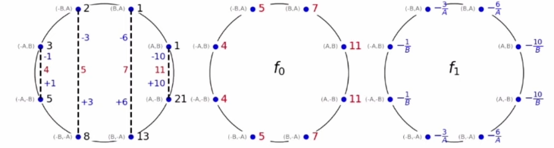
<figure><img src="https://755218234-files.gitbook.io/~/files/v0/b/gitbook-x-prod.appspot.com/o/spaces%2Frwz1ZAZJtK5FHz4Y1esA%2Fuploads%2Fgit-blob-de803679fdecc78146c3d3c963d246dd3c21afaa%2Fimage.png?alt=media" alt=""><figcaption><p>Figure 5. Given the evaluations (left), the result of <span class="math">J</span>-folding is shown. Notice that <span class="math">f_0</span> and <span class="math">f_1</span> can be actually parametrized by only the x-axis.</p></figcaption></figure>

($$\pi$$-folding) Next step:

$$
f\_{k\_00}(2\cdot x^2 - 1)=\frac{f\_{k\_0}(x) + f\_{k\_0}(-x)}{2}\f\_{k\_01}(2\cdot x^2 - 1)=\frac{f\_{k\_0}(x) - f\_{k\_0}(-x)}{2x}\f\_{k\_00}(2x^2 - 1) + xf\_{k\_01}(2x^2-1)=f\_{k\_0}(x)
$$

This step is repeated recursively until we get constant functions of the form:

$$
f\_{k\_0k\_1k\_2\dots k\_{n-1}}
$$

These make up a constant $$c\_k = f\_{k\_0,...,k\_{n−1}} \in F$$, for each $$k$$ in the interval $$0 \leq k \leq 2^{n} −1$$, where $$k = k\_0 + k\_1 2+. . .+k\_{n−1}2^{n−1}$$.

<figure><img src="https://755218234-files.gitbook.io/~/files/v0/b/gitbook-x-prod.appspot.com/o/spaces%2Frwz1ZAZJtK5FHz4Y1esA%2Fuploads%2FrNEvANUaUGUPWKYV10qM%2Fimage.png?alt=media&#x26;token=a1830b50-9d4f-4b4c-9018-22d658c8b4c3" alt=""><figcaption><p>Figure 6. Result of <span class="math">\pi</span>-folding on <span class="math">f_0</span>. We do the same for <span class="math">f_1</span> to get <span class="math">f_{10}</span> and <span class="math">f_{11}</span></p></figcaption></figure>

In Figure 6, $$f\_0(x)$$ suddenly has only 4 points. This is because $$f\_0(x)$$ actually has only 4 evaluation points $$(-A, -B, B, A)$$ and is only parametrized by $$x$$. It is visualized on a circle for easier group operation visualization. To elaborate:

1. $$f\_{00}(C)$$ is the average of $$f\_0(A)$$ and $$f\_0(-A)$$.
2. $$f\_{00}(-C)$$ is the average of $$f\_0(B)$$ and $$f\_0(-B)$$.

But where did $$C$$ come from? It denotes $$2A^2-1$$, while $$-C$$ is $$2B^2-1$$ since $$A^2 + B^2=1$$ because they are from a standard position coset.

**Theorem 2** Let $$p$$ be a CFFT-friendly prime supporting the order $$n\geq 1$$, take $$D \subset C(\mathbb{F}\_p)$$ a twin-coset of size $$|D| = 2^n$$. Given $$f \in F^D$$ a function over $$D$$ with values in an extension field $$F$$ of $$\mathbb{F}\_p$$ *,* the above described algorithm outputs the coefficients $$c\_k \in F$$, $$0 \leq k \leq 2^n-1$$, with respect to the FFT basis $$\mathcal{B\_n}$$, so that $$\sum^{2^n−1}{k=0}c\_k \cdot b\_k$$ evaluates to $$f$$ over $$D$$.

## Low degree test over the Circle

**Protocol 1 (Circle FRI)**. Let $$D$$ be a standard position coset of size $$|D| = 2^{B+n}$$, where $$B \geq 1$$ and $$n \geq 1$$, and let $$\mathcal{C} = \mathcal{C}\_N(F, D)$$ be the circle code with rate $$ho = \frac{N+1}{|D|}$$, where $$N = 2^n$$. For given proximity parameter $$\theta \in (0, 1 − \sqrt{ρ})$$, the interactive oracle proof of a function $$f \in F^D$$ being $$\theta$$-close to the circle code $$\mathcal{C}$$, consists of a commit phase and a subsequent query phase, which are as follows.

### **COMMIT** phase:

1. (Decomposition) The prover compute the decomposition of $$f\in\mathcal{L}\_N(F)$$ into $$f=f^{(0)} +\lambda\cdot v\_n$$ with $$f^{(0)}\in \mathcal{L}^{(0)}:=\mathcal{L}'\_N(F)$$ and $$\lambda\in F$$. It sends $$\lambda$$ and commitment to $$f^{(0)}$$ to the verifier.
2. ($$J$$-folding) For $$i = 1$$:
   1. The verifier picks uniformly random $$\beta\_i \in F$$ and sends it to the prover.
   2. The prover commits to a function $$f^{(i)}\in \mathcal{L}^{(i)}$$ (In the case of an honest prover, $$f^{(i)} = f^{(i-1)}*{0} + \beta\_i f^{(i-1)}*{1}$$ where\
      $$f^{(i-1)}\_0\circ\pi\_x=\frac{f^{(i-1)}+f^{(i-1)}\circ J}{2}\f^{(i-1)}\_1\circ\pi\_x=\frac{f^{(i-1)}-f^{(i-1)}\circ J}{2y}$$
3. ($$\pi$$-folding) For $$i = 2$$ to $$r$$:
   1. The verifier picks uniformly random $$\beta\_i \in F$$ and sends it to the prover.
   2. The prover commits to a function $$f^{(i)} : L^{(i)} \rightarrow F$$. (In the case of an honest prover, $$f^{(i)} = f^{(i-1)}*{0} + \beta\_i f^{(i-1)}*{1}$$ where

      $$f^{(i-1)}\_0\circ\pi=\frac{f^{(i-1)}+f^{(i-1)}\circ T}{2}\f^{(i-1)}\_0\circ\pi=\frac{f^{(i-1)}-f^{(i-1)}\circ T}{2x}$$

      where $$T(x)=-x$$.
4. The prover sends a value $$f^{(r)} \in \mathcal{L}^{(r)}$$ in plain.

### **QUERY** phase: (executed by the Verifier)

1. Repeat $$l$$ times where $$l$$ is the number of times you want to query to achieve target soundness:
   1. Pick $$x\_0 \in L^{(0)}$$ uniformly at random.
   2. ($$J$$-folding) For $$i = 1$$:
      1. Query $$f$$ at $$x\_0$$ and $$J(x\_0)$$. Compute \
         $$f^{(0)}(x\_0)=f(x\_0)-\lambda\cdot v\_n(x\_0)\f^{(0)}(J(x\_0))=f(J(x\_0)) - \lambda\cdot v\_n(J(x\_0))$$
      2. Compute\
         &#x20;$$f^{(0)}\_0(\pi\_x(x\_0)) = \frac{f^{(0)}(x\_0) + f^{(0)}(J(x\_0))}{2}\f^{(0)}\_1(\pi\_x(x\_0)) = \frac{f^{(0)}(x\_0) + f^{(0)}(J(x\_0))}{2y}$$
      3. Query $$f^{(1)}$$ at $$x\_1=\pi\_x(x\_0)$$ and check if \
         $$f^{(1)}(\pi\_x(x\_0)) = f^{(0)}*{0}(\pi\_x(x\_0)) + \beta\_1 f^{(0)}*{1}(\pi\_x(x\_0))$$
   3. ($$\pi$$-folding) For $$i = 2\dots r$$:
      1. Calculate $$x\_i=\pi(x\_{i-1})=2x^2\_{i-1}-1$$
      2. Query $$f^{(i-1)}$$ at $$-x\_{i-1}$$. (the value at $$x\_{i-1}$$ is queried in the previous round)
      3. Compute\
         $$f^{(i-1)}*0(x\_i) = \frac{f^{(i-1)}(x*{i-1}) + f^{(i-1)}(-x\_{i-1})}{2}\f^{(i-1)}*1(x\_i) = \frac{f^{(i-1)}(x*{i-1}) - f^{(i-1)}(-x\_{i-1}))}{2x\_{i-1}}$$
      4. Query $$f^{(i)}$$ at $$x\_i$$ and check if\
         $$f^{(i)}(x\_i) = f^{(i-1)}*{0}(x\_i) + \beta\_i f^{(i-1)}*{1}(x\_i)$$
2. ACCEPT if all checks passed. REJECT otherwise

### Batch Circle FRI

**Protocol 2 (batch Circle FRI).** Under the same assumptions as Protocol 1, the interactive oracle proof for a batch of functions $$f\_1,\dots,f\_L \in F^D$$ having correlated $$(1 − \theta)$$-agreement to a codeword from $$C\_N(F, D)$$, is as follows. In the first step, given a random challenge $$\lambda\_b \leftarrow F$$ from the verifier, the prover computes the values of the linear combination:

$$
f=\sum^L\_{i=1}\lambda\_b^{k-1}\cdot f\_i
$$

over $$D$$. Now, both prover and verifier run Protocol 1 on $$f$$ , with its query phase extended by a check of the batching at each of the queries.

## CircleSTARK

In circle STARK, the **trace domain** is the standard position coset $$H\subset C(\mathbb{F}\_p)$$ of a cyclic and proper subgroup $$G = G\_n$$ of the circle curve $$C(\mathbb{F}\_p)$$, of size $$N = 2^n$$, with $$n \geq 1$$, and the trace is organised column-wise $$t\_1, \dots, t\_w \in \mathbb{F}\_p^N$$, each placed over the domain $$H$$ in the usual manner, using the group translation $$T$$ by a generator of $$G$$ for the timeline. The trace columns are interpolated by polynomials

$$
p\_1,\dots,p\_w\in\mathbb{F}\_p\[x,y]/(x^2+y^2 -1)
$$

of total degree at most $$N/2$$, meaning that $$p\_i\in\mathcal{L}\_N(\mathbb{F}\_p)$$ (actually, they are from the FFT-space $$\mathcal{L}'\_N(\mathbb{F}\_p))$$, and these polynomials are subject to set of constraints, say

$$
P\_i(s\_i,p\_1,\dots,p\_w,p\_1\circ T,\dots,p\_w\circ T)=0
$$

for $$i=1,\dots,C$$, holding over the entire domain $$H$$, where $$s\_i\in \mathcal{L}\_N(\mathbb{F}\_p)$$ is a predefined selector polynomial.

Each constraint is a polynomial

$$
P\_i\in\mathbb{F}\_p\[S,X\_1,\dots,X\_w,Y\_1,\dots,Y\_w]
$$

$$P\_i\in\mathbb{F}\_p\[S,X\_1,\dots,X\_w,Y\_1,\dots,Y\_w]$$of total degree at most the maximum number of twin-coset of size $$N$$, $$\mathsf{deg} P\_i\leq\frac{p^2+1}{N} - 1$$ and the degree in the selector variable $$S$$ is at most $$\mathsf{deg}\_S P\_i \leq 1$$.

**Definition.** The **evaluation domain** is a standard position coset $$D\subseteq C(\mathbb{F}\_p)$$, of at least double the size of trace domain $$H$$. The polynomials in the circle STARK will be generally committed by their values over this domain.

**Lemma 2 from the paper**. Let $$p$$ be a CFFT-friendly prime supporting the order $$m \geq 1$$, and $$G\_k$$ denote the subgroup of order $$2^k$$ for $$k \leq m$$. Then any subset of $$D\subseteq C(\mathbb{F}\_p) / G\_m$$ which is invariant under and $$J$$ can be decomposed into twin-cosets of size $$N = 2^n$$, for any $$n \leq m$$. In particular for a standard position coset $$D$$ of size $$M = 2^m$$,

$$
D = Q \cdot G\_m = \bigcup^{M/N-1}*{k=0}(Q^{4k+1}\cdot G*{n−1} \cup Q^{−4k−1}\cdot G\_{n−1})
$$

where $$Q$$ is an element from $$C(\mathbb{F}\_p)$$ of order $$2^{m+1}$$.

### IOP for AIR

Now, once we have all these, the interactive oracle proof for the satisfiability of the AIR can be constructed as follows:

In the first round, the prover computes the values of its trace polynomials $$p\_1,\dots,p\_w\in\mathcal{L}\_N(\mathbb{F}\_p)$$ over the evaluation domain $$D$$ using its decomposition into twin-cosets and shares their oracles denoted by

$$
\[p\_1],\dots,\[p\_w]
$$

with their verifier.

In the second round, the verifier sends random challenge $$\beta \leftarrow F$$, drawn uniformly from a suitably large extension field $$F$$ of $$\mathbb{F}\_p$$, which is used to reduce the constraint polynomials into a single one:

$$
\sum^C\_{i=1}\beta^{i-1}\cdot P\_i(s\_i,p\_1,\dots,p\_w,p\_1\circ T,\dots,p\_w\circ T)=0
$$

which should hold over trace domain $$H$$. To prove this, the vanishing polynomial over $$H$$, $$v\_H$$, is computed so the composite constraint polynomial can now be written as:

$$
\sum^C\_{i=1}\beta^{i-1}\cdot P\_i(s\_i,p\_1,\dots,p\_w,p\_1\circ T,\dots,p\_w\circ T)=q\cdot v\_H
$$

To keep with the degree bound imposed by the size of $$H$$, the quotient $$q\in\mathcal{L}*{(d-1)N}(F)$$ needs to be split into polynomials $$q\_1,\dots,q*{d-1}\in\mathcal{L}\_N(F)$$:

$$
q=\lambda\cdot v\_{\bar H} + \sum^{d-1}*{k=1}\frac{v*{\bar H}}{v\_{H\_k}}\cdot q\_k
$$

Recall that $$L\_{(d-1)N}$$ has $$(d-1)N + 1$$ dimension. On the other hand, the quotient $$q\in\mathcal{L}*{(d-1)N}(F)$$ is computed by value from those of $$f\_1,\dots,f\_w$$ over a union of twin-cosets $$H\_k$$ of size $$N$$. Thus the union $$\bar{H}=\bigcup^{d-1}*{k=1}H\_k$$ is one point too small to uniquely determine a polynomial from $$\mathcal{L}\_{(d-1)N}$$. In our decomposition, this missing point is characterized by an additional scalar multiple of the vanishing polynomial of $$\bar{H}$$.

Then, the prover sets up the oracles

$$
\[q\_1],\dots,\[q\_{d-1}]
$$

for their values over the evaluation domain $$D$$, and sends them, together with $$\lambda$$, to the verifier.

Having all oracles in place, the next step is DEEP ALI, which reduces satisfiability of the constraints to a low-degree test on single-point quotients. (In lose terms, this step turns low-degree test into a polynomial commitment scheme.)

In this step, the verifier responds with a random point $$\gamma\rightarrow C(F)\setminus (D\cup H)$$. In return, the prover opens the values $$v\_{i,0}=p\_i(\gamma), v\_{i,1}=p\_i(T(\gamma))$$ for each $$i=1,\dots,w$$ as well as $$v\_1,\dots,v\_{d-1}$$ of $$q\_1,\dots,q\_{d-1}$$ at $$\gamma$$. Eventually, both prover and verifier engage in a low-degree test for the real and imaginary parts of the DEEP quotients:

$$
\mathsf{Re/Im}(\frac{p\_i-v\_{i,0}}{v\_\gamma}),\mathsf{Re/Im}(\frac{p\_i-v\_{i,1}}{v\_{T(\gamma)}})\\\mathsf{Re/Im}(\frac{q\_i-v\_i}{v\_\gamma})
$$

## Conclusion

The initial implementation of CircleFFT demonstrated a performance improvement by a factor of 1.4 in a single-threaded setup. Building on this foundation, Starknet’s next-generation prover, Stwo (“STARK Two”), is designed to enhance and eventually replace the current prover, Stone (“STARK One”).

<figure><img src="https://755218234-files.gitbook.io/~/files/v0/b/gitbook-x-prod.appspot.com/o/spaces%2Frwz1ZAZJtK5FHz4Y1esA%2Fuploads%2F8SbPlyL4kn3NaOMKaJid%2Fimage.png?alt=media&#x26;token=b7dc1b94-abe8-4c4f-a930-472eca7e675b" alt=""><figcaption><p>Figure 7. Initial benchmark result of CFFT</p></figcaption></figure>

> Written by [Batzorig Zorigoo](https://app.gitbook.com/u/cO1lUla01ZW0seepO37jMHFTxg42 "mention") of Fractalyze