# Binius

## **Introduction**

In recent STARKs, there has been a trend of using smaller fields to achieve faster performance, such as **Goldilocks** (64-bit) and smaller 32-bit fields like **Baby Bear** and **Mersenne 31**. Naturally, this leads to the question: *Can we use the smallest field, the **binary field**?*

Given that computers are optimized for bit operations, using a binary field could promise better performance. Additionally, if we can express constraints efficiently using the binary field, this would allow us to handle binary operations in commonly used hash functions like **Keccak** more effectively.

While the [STARK](https://eprint.iacr.org/2018/046) paper attempted to use binary fields, it faced challenges:

1. The binary field was too small to serve as an "alphabet" in Reed-Solomon (RS) codes compared to the block length, necessitating embedding.
2. As noted in [HyperPlonk](https://eprint.iacr.org/2022/1355), using a shift function to traverse the entire evaluation domain introduced overhead.

This article will explore how [**Binius**](https://eprint.iacr.org/2023/1784) overcomes these issues.

## Background

### Embedding Overhead

**Embedding overhead** refers to the inefficiency caused when representing values smaller than a given field $$\mathbb{F}$$ and filling the space difference with zero padding or similar techniques. This overhead often occurs during range checks or when binary operations are arithmetized. [For example, in the Keccak-256 circuit, out of 2,531 columns, 2,328 columns each represent a single bit, but since each column can hold up to 64 bits, there is a massive embedding overhead.](https://youtu.be/BeEuphrUipk?t=302)

### Binary Field

Addition in a binary field operates as follows:

$$
0 + 0 \equiv 0 \pmod 2 \\
0 + 1 \equiv 1 \pmod 2 \\
1 + 0 \equiv 1 \pmod 2 \\
1 + 1 \equiv 0 \pmod 2 \\
$$

This is equivalent to the **XOR operation**. Since x + (-x) = 0 defines -x as the negative of x, and 0 + 0 = 0 and 1 + 1 = 0, the negative of any element in a binary field is the element itself. In other words, subtraction is equivalent to addition:

$$
0 - 0 = 0 + 0 \equiv 0 \pmod 2 \\
0 - 1 = 0 + 1 \equiv 1 \pmod 2 \\
1 - 0 = 1 + 0 \equiv 1 \pmod 2 \\
1 - 1 = 1 + 1 \equiv 0 \pmod 2
$$

Furthermore, a **doubling operation** such as $$2 \cdot a$$ always equals 0, since it becomes a multiple of 2. Multiplication in a binary field is therefore defined as follows:

$$
0 \cdot 0 \equiv 0 \pmod 2 \\
0 \cdot 1 \equiv 0 \pmod 2 \\
1 \cdot 0 \equiv 0 \pmod 2 \\
1 \cdot 1 \equiv 1 \pmod 2
$$

This is equivalent to the **AND operation**.

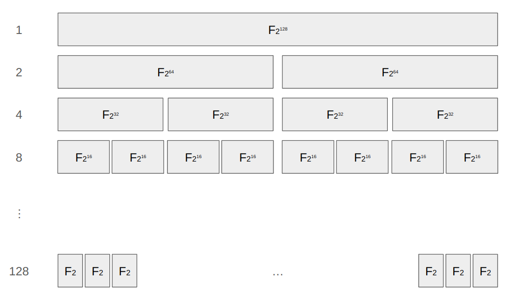
#### Binary Tower <a href="#binary-tower" id="binary-tower"></a>

A **binary tower** is a hierarchical structure of finite fields, where each field in the hierarchy is an extension of the previous field, and the base field is $$\mathbb{F}\_2$$​. In [An Iterated Quadratic Extension of GF(2)](https://www.fq.math.ca/Scanned/26-4/wiedemann.pdf), it is stated that an extension field can be constructed as

$$
T\_0 := \mathbb{F}*2 \T\_1 := T\_0\[X\_0] / (X\_0^2 + X\_0 + 1) \cong \mathbb{F}*{2^2}\T\_2 := T\_1\[X\_1] / (X\_1^2 + X\_1  X\_0 + 1) \cong \mathbb{F}*{2^4} \T\_3 := T\_2\[X\_2] / (X\_2^2 + X\_2 X\_1 + 1) \cong \mathbb{F}*{2^8}\\
\cdots \T\_\iota  := T\_{\iota - 1}\[X\_{\iota - 1}] / (X\_{\iota-1}^2 + X\_{\iota-1} X\_{\iota - 2} + 1) \cong \mathbb{F}\_{2^{2^\iota}}
$$

This can be illustrated as follows:

<figure><img src="https://files.gitbook.com/v0/b/gitbook-x-prod.appspot.com/o/spaces%2FHFUA8ip5LfWrOBM4eFfr%2Fuploads%2FumzxRZaUXt14kpcdtmNz%2Fimage.png?alt=media&#x26;token=8622e9c3-4411-41aa-a5ea-aef4ab0c0481" alt=""><figcaption></figcaption></figure>

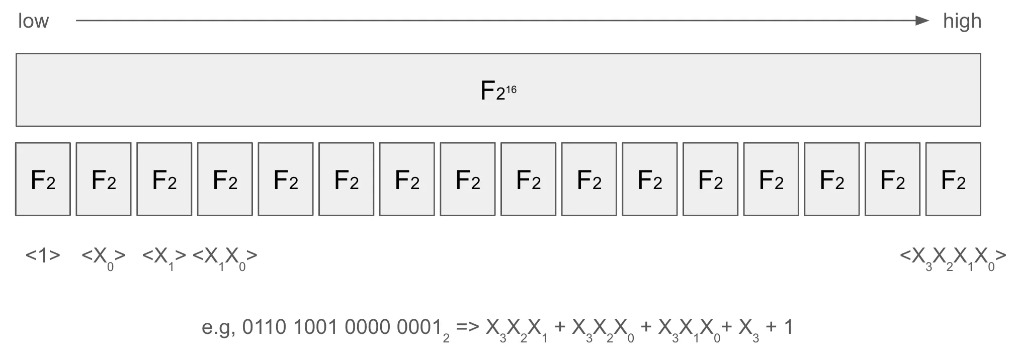
For example, let’s represent **135** using a **binary tower**. Here, $$X\_2$$ corresponds to $$2^4$$, $$X\_1$$ ​corresponds to $$2^2$$, and $$X\_0$$​ corresponds to $$2$$:

$$
135
\=X\_2X\_1X\_0 + X\_1 + X\_0 + 1 \because 135 = 2^4\cdot2^2\cdot2 + 2^2 + 2 +1 \\
$$

By continually substituting $$X\_i$$​ with $$X\_{i-1}$$​, we can transform it into the form of a **multilinear polynomial**:

$$
\begin{align\*}
& h X\_1 + l \in T\_2 \cong \mathbb{F}*{2^4} \text{, where }h,l \in T\_1 \cong \mathbb{F}*{2^2} \\
&= (h\_1X\_0 + h\_2)X\_1 + (l\_1X\_0 + l\_2) \\
&= h\_1X\_1X\_0 + h\_2X\_1 +l\_1X\_0 + l\_2\text{, where } h\_i, l\_i \in T\_0 \cong \mathbb{F}\_2 \\
\end{align\*}
$$

The equation above shows how we can transform a case of $$T\_2$$ to a multilinear polynomial, while the equation below shows how we can transform a case of $$T\_3$$ to a multilinear polynomial.

$$
\begin{align\*}
& hX\_2 + l \in T\_3 \cong \mathbb{F}*{2^8} \text{, where } h, l \in T\_2 \cong \mathbb{F}*{2^4} \\
&= (h\_1X\_1 + h\_2)X\_2 + l\_1X\_1 + l\_2 \text{, where } h\_i, l\_i \in T\_1 \cong \mathbb{F}\_{2^2} \text{ if } i \le 2  \\
&= ((h\_3X\_0 + h\_4)X\_1 + h\_5X\_0 + h\_6)X\_2 + (l\_3X\_0 + l\_4)X\_1 + l\_5X\_0 + l\_6 \\
&= h\_3X\_2X\_1X\_0 + h\_4X\_2X\_1 + h\_5X\_2X\_0+h\_6X\_2+l\_3X\_1X\_0 + l\_4X\_1 + l\_5X\_0 + l\_6 \text{,} \ &\text{where } h\_i, l\_i \in T\_0 \cong \mathbb{F}\_2 \text{ if } i > 2
\end{align\*}
$$

This allows for the **canonical mapping of bitstrings**. (For example, in $$\mathbb{F}\_7$$ the 3-bit space maps both 0 and 7 to 0.)

$$
v = \sum\_{i = 0}^{2^i - 1} b\_i \cdot 2^i
$$

Here, the set of $$b\_i$$ are coefficients of a multilinear polynomial.

In the extension field, **addition** can be performed using **XOR** as in the binary field. However, for **multiplication**, the following steps must be used:

1. Multiply both sides (for $$i \geq 0$$):

$$
(aX\_i + b)(cX\_i + d) = ac{X\_i}^2 + (ad + bc)X\_i + bd
$$

2. Substitute $${X\_i}^2$$ with $$X\_{i-1}X\_i + ac$$:

$$
ac{X\_i}^2 + (ad + bc)X\_i + bd = (ad + bc + acX\_{i-1})X\_i + ac + bd
$$

3. If $$i - 1 = 0$$, stop. Otherwise, repeat the process for $$ac$$, $$ad$$, $$bc$$, and $$bd$$.

Notably, using the [**Karatsuba algorithm**](https://en.wikipedia.org/wiki/Karatsuba_algorithm), the number of multiplications can be reduced from 4 to 3:

$$
(aX\_i + b)(cX\_i + d) = ((a + b)(c + d) - ac - bd + acX\_{i-1})X\_i + ac + bd
$$

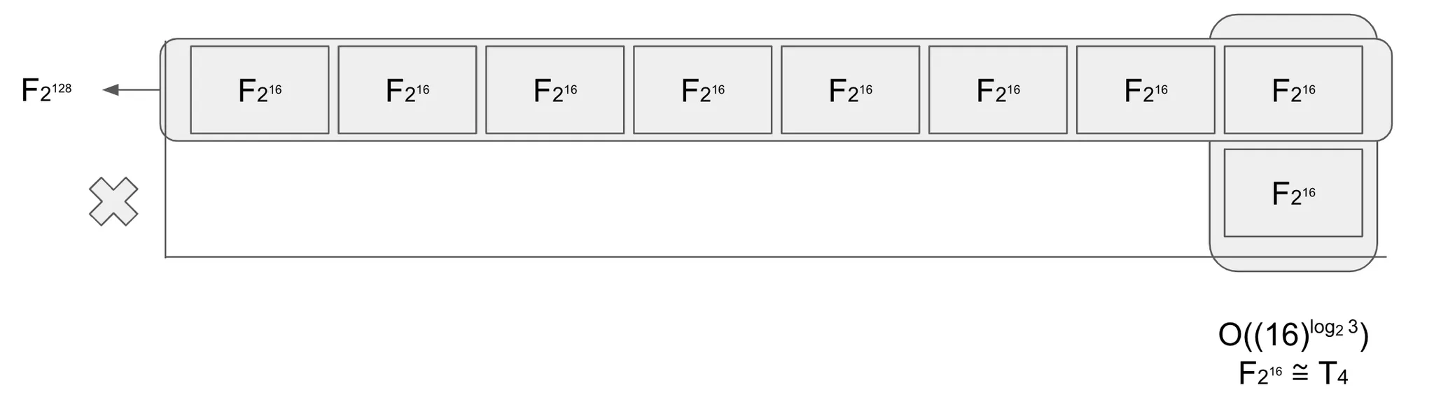
According to [On efficient inversion in tower fields of characteristic two](https://ieeexplore.ieee.org/document/612935), multiplication with this binary tower structure can be computed in $$\Theta((2^i)^{log\_2 3})$$.

Note that the **classic method** for constructing extension fields is as follows:

$$
\mathbb{F}\_{2^{128}} := \mathbb{F}\_2\[X] / f(X)\text{, where } f(X) \text{ is irreducible and } \deg f(X) = 128
$$

In this extension field, addition is still computed using **XOR**. For multiplication, polynomials of degree 127 are multiplied and then divided by $$f(X)$$.

Using Binary Towers for extension field operations provides an advantage over doing so with the classic method due to the following reasons:

* In circuits, various data sizes (e.g., bits) can be represented efficiently with Binary Towers.
* When expressing $$\mathbb{F}\_{2^{16}}$$ using 16 instances of $$\mathbb{F}\_2$$​, efficient **embedding** methods (packing) are available. In contrast, classic methods [depend on the choice of an irreducible ](#user-content-fn-1)[^1]polynomial and are often less efficient.

  <figure><img src="https://755218234-files.gitbook.io/~/files/v0/b/gitbook-x-prod.appspot.com/o/spaces%2Frwz1ZAZJtK5FHz4Y1esA%2Fuploads%2Fgit-blob-eef3b2463736ec0de6f344a26979f805def60113%2Fimage.png?alt=media" alt=""><figcaption></figcaption></figure>
* Multiplying an element of $$\mathbb{F}*{2^{16}}$$ with an element of $$\mathbb{F}*{2^{128}}$$ is faster than multiplying two elements of $$\mathbb{F}*{2^{128}}$$. The cost is $$8 \cdot \Theta(16^{\log\_2 3})$$. In contrast, classic methods require embedding $$\mathbb{F}*{2^{16}}$$​ into $$\mathbb{F}\_{2^{128}}$$​, making them slower.

  <figure><img src="https://755218234-files.gitbook.io/~/files/v0/b/gitbook-x-prod.appspot.com/o/spaces%2Frwz1ZAZJtK5FHz4Y1esA%2Fuploads%2Fgit-blob-19594a1b50b207d512c972877b6a010aaa9a74a3%2Fimage.png?alt=media" alt=""><figcaption></figcaption></figure>

## **Protocol Explanation**

### **Block-level Encoding-based PCS**

In **Brakedown**, instead of Reed-Solomon (RS) codes, linear codes with linear encoding time are used. In comparison, **Binius** adopts the overall style of Brakedown while leveraging **RS codes** with the [**Singleton bound**](https://en.wikipedia.org/wiki/Singleton_bound), which states that the maximum distance for $$\[n, k, d]$$-codes is $$d \leq n - k + 1$$. Furthermore, instead of using [radix-2 FFT](https://en.wikipedia.org/wiki/Cooley%E2%80%93Tukey_FFT_algorithm#The_radix-2_DIT_case) for RS encoding in a binary field, **additive FFT** ([paper](https://arxiv.org/pdf/1404.3458)) is used; however, the size of the alphabet must be at least $$n$$, but the size of the alphabet $$\mathbb{F}*2$$​ is far smaller than $$n$$. To address this, we construct $$\mathbb{F}*{2^{16}}$$​ using, for example, 16 instances of $$\mathbb{F}*2$$​. This method is called **packing**. Since the encoding is performed in blocks of $$\mathbb{F}*{2^{16}}$$​, this is referred to as **block-level encoding**.

$$g(X\_0, \dots, X\_{l-1}) \in T\_{\iota}\[X\_0, \dots, X\_{l-1}]^{\le1}$$ and evaluation point $$\bm{r} = (r\_0, \dots, r\_{l-1}) \in T\_\tau^l$$, let $$t$$ be an $$(m\_0 = 2^{l\_0}) \times (m\_1 = 2^{l\_1})$$ matrix consisting of the coefficients in the multilinear Lagrange basis. (For simplicity, let $$\iota = 0, \kappa = 4, \tau = 7$$.  As aforementioned in the Binary Towers section, $$T\_\iota = \mathbb{F}*{2}, T*\kappa = \mathbb{F}*{2^{16}}, T*\tau = \mathbb{F}\_{2^{128}}$$. The evaluation $$g(\bm{r})$$ can then be computed as follows:

$$
g(\bm{r}) = \otimes\_{i = l\_1}^{l - 1}(1 - r\_i, r\_i)\cdot (t\_i)*{i=0}^{m\_0 - 1} \cdot \otimes*{i = 0}^{l\_1 - 1}(1 - r\_i, r\_i)
$$

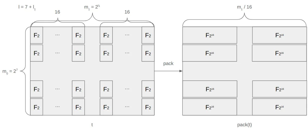
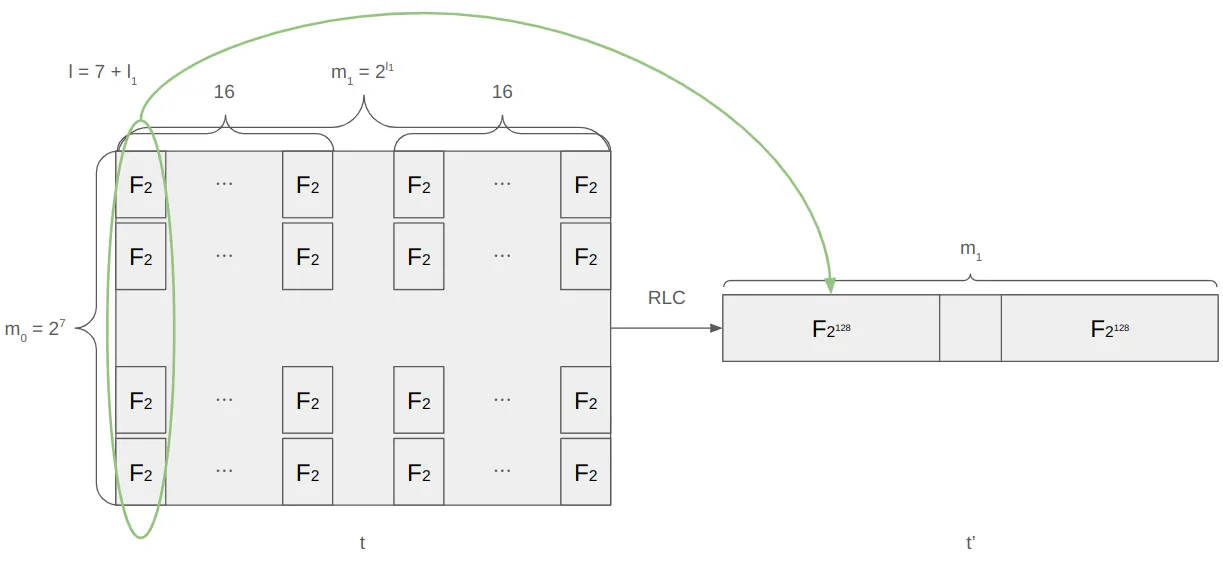
Here, $$l = (l\_0 = 7) + l\_1$$, and $$\bm{t\_i} \in (T\_\iota^{m\_1})^{m\_0}$$ is the $$i$$-th row of $$\bm{t}$$.

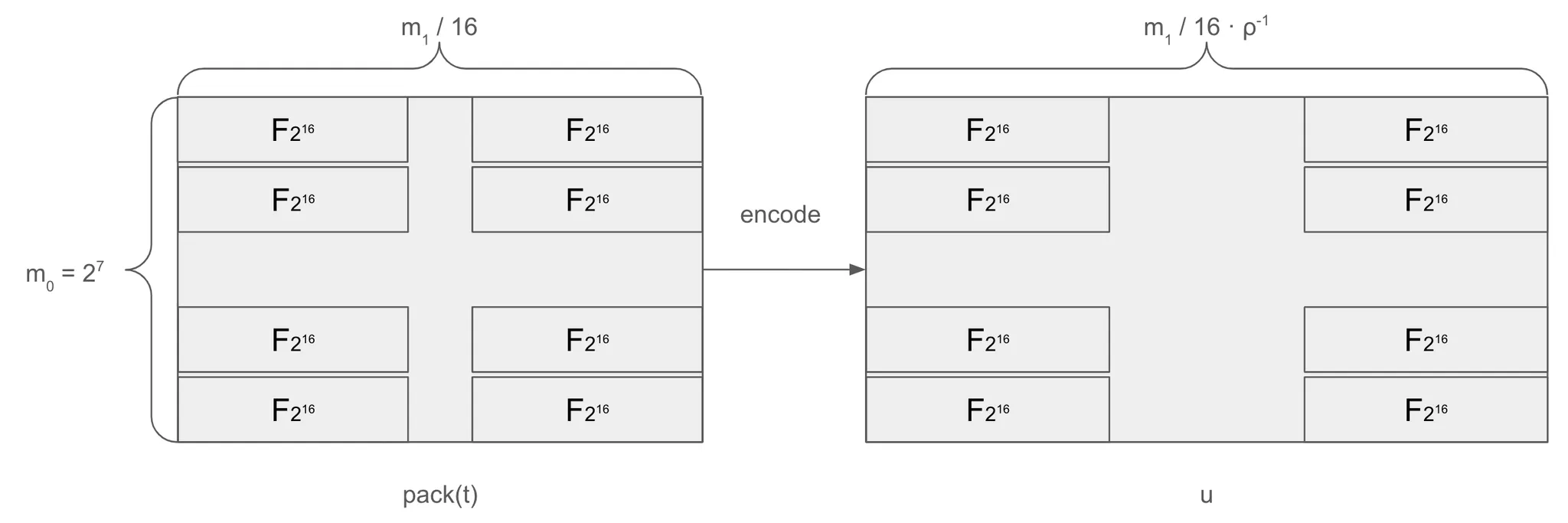
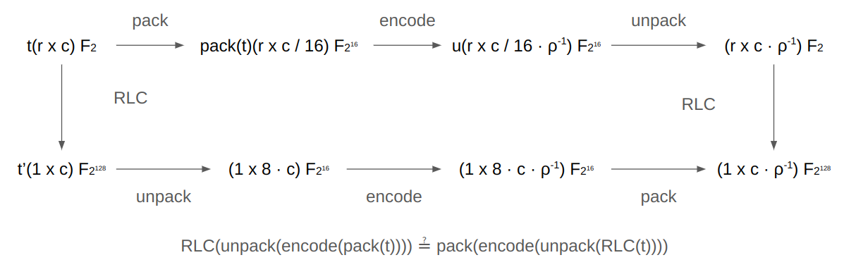
1. From the $$m\_0 \times m\_1$$ ​matrix $$\bm{t}$$, pack each row of length $$m\_1$$ ​into a new $$m\_0 \times \frac{m\_1}{2^\kappa}$$ matrix $$\mathsf{pack}(\bm{t})$$.

   <figure><img src="https://755218234-files.gitbook.io/~/files/v0/b/gitbook-x-prod.appspot.com/o/spaces%2Frwz1ZAZJtK5FHz4Y1esA%2Fuploads%2Fgit-blob-6a36843b2678fb927f1dadc8542dc497f5f6977b%2Fimage.png?alt=media" alt=""><figcaption></figcaption></figure>
2. If the rate is $$\rho$$, encode each row of the $$m\_0 \times \frac{m\_1}{2^\kappa}$$ matrix $$\mathsf{pack}(\bm{t})$$ into rows of length $$n = \frac{m\_1}{2^\kappa}\cdot\rho^{-1}$$, forming an $$m\_0 \times n$$ matrix $$u$$. The prover sends a Merkle hash-based commitment of the $$u$$ matrix to the verifier. Note that while the polynomial represented by the $$\bm{t}$$ matrix is $$g$$, the polynomial represented by $$\mathsf{pack}(\bm{t})$$ is a new polynomial $$g'$$.<br>

   <figure><img src="https://755218234-files.gitbook.io/~/files/v0/b/gitbook-x-prod.appspot.com/o/spaces%2Frwz1ZAZJtK5FHz4Y1esA%2Fuploads%2Fgit-blob-1637f6ee981673428b1ff43182932df3ca71200a%2Fimage.png?alt=media" alt=""><figcaption></figcaption></figure>
3. The verifier samples $$\bm{r} = (r\_0, \dots,r\_{l-1}) \leftarrow \mathbb{F\_{2^{128}}^l}$$​ and sends it to the prover.
4. The prover computes $$s = g(r\_0, \dots, r\_{l-1})$$ and $$\bm{t'} = \otimes\_{i = l\_1}^{l-1}(1 - r\_i, r\_i)\cdot (\bm{t\_i})*{i = 0}^{m\_0 - 1}$$, and sends both to the verifier. Note that $$\bm{r}$$ is over $$\mathbb{F}*{2^{128}}$$, $$\bm{t}$$ is over $$\mathbb{F}*2$$​, and $$\bm{t'}$$ is over $$\mathbb{F}*{2^{128}}$$. As mentioned in Binary Towers, multiplication in this setting is performed efficiently.

   <figure><img src="https://755218234-files.gitbook.io/~/files/v0/b/gitbook-x-prod.appspot.com/o/spaces%2Frwz1ZAZJtK5FHz4Y1esA%2Fuploads%2Fgit-blob-0d9207d26e1fe0b895761841b03e9d3e376fac8d%2Fimage.png?alt=media" alt=""><figcaption></figcaption></figure>
5. The verifier samples $$j\_i \leftarrow {0, \dots, n - 1}$$ for $$\gamma$$ times, where $$\gamma$$ is the repetition count, and sends $$\bm{J} = {j\_0, \dots, j\_{\gamma - 1}}$$ to the prover (Remember $$n = \frac{m\_1}{2^\kappa}\cdot\rho^{-1}$$).
6. The verifier uses Merkle proofs to verify that $$\big{(u\_{i, j})\big}\_{j \in \bm{J}}$$​ is correct.
7. Finally, the verifier checks that packing and encoding were performed correctly:\
   . Given that $$j\_i$$​ ranges between $$0$$ and $$n = \frac{c}{16} \cdot \rho^{-1}$$, testing is performed at the **block level** in units of $$\mathbb{F}\_{2^{16}}$$​. This is referred to as **block-level testing**.

   <figure><img src="https://755218234-files.gitbook.io/~/files/v0/b/gitbook-x-prod.appspot.com/o/spaces%2Frwz1ZAZJtK5FHz4Y1esA%2Fuploads%2Fgit-blob-57b94fceeb58fe0d84de13c597afd0078c5e27a2%2Fimage.png?alt=media" alt=""><figcaption></figcaption></figure>

### Pack Virtual Polynomial

Let us revisit the block-level encoding described earlier. In a **Polynomial IOP**, the polynomial that the verifier requests the prover to open is $$g \in \mathbb{F}*2\[X\_0, \dots, X*{l-1}]^{\leq 1}$$. However, the polynomial that the prover actually commits to and opens is $$g'$$, which is derived by packing $$g$$ into $$g' \in \mathbb{F}*{2^{\kappa}}\[X\_0, \dots, X*{l - \kappa - 1}]^{\leq 1}$$. The **packing function** $$\widetilde{\mathsf{pack}}\_{\kappa}$$​ is defined as follows:<br>

$$
\widetilde{\mathsf{pack}}*{\kappa}(g)(X\_0, \dots, X*{l - \kappa - 1}) :=\sum\_{v\in B\_\kappa}\tilde{g}(v\_0, \dots, v\_{\kappa - 1}, X\_0, \dots, X\_{l - \kappa - 1}) \cdot \beta\_v
$$

Here, $$\tilde{g}$$ is the multilinear extension (MLE) of $$g$$, and $$\beta\_v$$ represents the multilinear Lagrange basis. For example, when $$\kappa = 2$$ and $$l = 4$$, the equation becomes:

$$
\begin{align\*}
\widetilde{\mathsf{pack}}\_2(g)(X\_0, X\_1) =&\tilde{g}(1, 1, X\_0, X\_1)\cdot 8 +   \tilde{g}(0, 1, X\_0, X\_1)\cdot 4 + \\
&\tilde{g}(1, 0, X\_0, X\_1)\cdot 2 + \tilde{g}(0, 0, X\_0, X\_1)\cdot 1
\end{align\*}
$$

Using a **sumcheck protocol**, this computation can be replaced with an evaluation claim such that:

$$
\widetilde{\mathsf{pack}}\_\kappa(g)(\bm{r'}) \stackrel{?}= s'
$$

Replacing $$\beta\_v$$ with $$\tilde{\beta} \in \mathbb{F}*\kappa\[X\_0, \dots, X*{\kappa - 1}]^{\le 1}$$, the following equation is defined:

$$
\widetilde{\mathsf{pack}}*{\kappa}(g)(\bm{r'})(Y\_0, \dots, Y*{\kappa - 1}) := \tilde{g}(Y\_0, \dots, Y\_{\kappa - 1}, {r'}*0, \dots, {r'}*{l - \kappa - 1}) \cdot \tilde{\beta}(Y\_0, \dots, Y\_{\kappa - 1})
$$

The following sum holds:

$$
\sum\_{Y \in B\_{ \kappa}}\widetilde{\mathsf{pack}}*{\kappa}(g)(\bm{r'})(Y\_0, \dots, Y*{\kappa - 1}) = s'
$$

For example, when $$\kappa = 2$$:

$$
\begin{align\*} \widetilde{\mathsf{pack}}\_2(g)(\bm{r'}) = s' =&\tilde{g}(1, 1, {r'}\_0, {r'}\_1)\cdot Y\_1Y\_0 + \tilde{g}(0, 1, {r'}\_0, {r'}\_1)\cdot Y\_1 + \ &\tilde{g}(1, 0, {r'}\_0, {r'}\_1)\cdot Y\_0 + \tilde{g}(0, 0, {r'}\_0, {r'}\_1)\cdot 1 \end{align\*}
$$

By applying a **sumcheck protocol**, this is replaced with an evaluation claim:

$$
\tilde{g}(\bm{r} || \bm{r'}) \cdot \tilde{\beta}(\bm{r}) \stackrel{?}= s
$$

Thus, we obtain $$\tilde{g}(\bm{r} || \bm{r'})$$, allowing us to query the original polynomial $$g$$ through its **virtual polynomial** $$g'$$.

### Shift Virtual Polynomial

As introduced in the previous article on **HyperPlonk**, the **shift polynomial** helps traverse the evaluation domain. For $$\bm{b} \in {0, \dots, l-1}$$ and shift offset $$o \in B\_b$$​, the **shift mapping** $$s\_{b, o}: B\_l \rightarrow B\_l$$​ is defined such that, for $$u := s\_{b, o}(v)$$, the condition $${u} \equiv {v} + {o} \pmod{2^b}$$ holds. For example, shifting by $$o = {1, 0} \in B\_2$$​ (a single step) works as follows:

$$
s\_{b, o}(0, 0, 0) = (1, 0, 0) \\
s\_{b, o}(1, 0, 0) = (0, 1, 0) \\
s\_{b, o}(0, 1, 0) = (1, 1, 0) \\
s\_{b, o}(1, 1, 0) = (0, 0, 0) \\
s\_{b, o}(0, 0, 1) = (1, 0, 1) \\
s\_{b, o}(1, 0, 1) = (0, 1, 1) \\
s\_{b, o}(0, 1, 1) = (1, 1, 1) \\
s\_{b, o}(1, 1, 1) = (0, 0, 1) \\
$$

The **shift operator** is defined as:

$$
\text{shift}*{b, o}(g) := g\circ s*{b,o}
$$

The **shift indicator** $$\text{s-ind}\_{b, o}$$​ can be expressed as follows: (Refer to the section 4.3. in the paper to see how it is algebraically expressed)

$$
\text{s-ind}\_{b, o}(x, y) \rightarrow \begin{cases}
1& \text{if } {y} \stackrel{?}\equiv {x} + {o} \pmod{2^b}\ 0 &\text{otherwise} \end{cases}
$$

Thus, the **shift polynomial** $$\widetilde{\mathsf{shift}}\_{b, o}(g)$$ is defined as:

$$
\widetilde{\text{shift}}*{b, o}(g)(\bm{v}) := \sum*{u \in B\_b}\tilde{g}(u\_0, \dots, u\_{b-1}, v\_b, \dots, v\_{l-1})\cdot \widetilde{\text{s-ind}}*{b, o}(u\_0, \dots, u*{b-1}, v\_0, \dots, v\_{b-1})
$$

For the earlier example:

$$
\widetilde{\text{shift}}*{b, o}(g)(0, 0, 0) = \tilde{g}(1, 0, 0) \\
\widetilde{\text{shift}}*{b, o}(g)(1, 0, 0) = \tilde{g}(0, 1, 0) \\
\widetilde{\text{shift}}*{b, o}(g)(0, 1, 0) = \tilde{g}(1, 1, 0) \\
\widetilde{\text{shift}}*{b, o}(g)(1, 1, 0) = \tilde{g}(0, 0, 0) \\
\widetilde{\text{shift}}*{b, o}(g)(0, 0, 1) = \tilde{g}(1, 0, 1) \\
\widetilde{\text{shift}}*{b, o}(g)(1, 0, 1) = \tilde{g}(0, 1, 1) \\
\widetilde{\text{shift}}*{b, o}(g)(0, 1, 1) = \tilde{g}(1, 1, 1) \\
\widetilde{\text{shift}}*{b, o}(g)(1, 1, 1) = \tilde{g}(0, 0, 1) \\
$$

By applying the **sumcheck protocol**, we get the evaluation claim:

$$
\widetilde{\text{shift}}\_{b,o}(g)(\bm{r'}) \stackrel{?}= s'
$$

This leads to:

$$
\widetilde{\text{shift}}*{b,o}(g)(\bm{r'})(Y\_0, \dots, Y*{b- 1}) := \tilde{g}(Y\_0, \dots, Y\_{b- 1}, {r'}*b, \dots, {r'}*{l - 1}) \cdot \widetilde{\text{s-ind}}*{b,o}(Y\_0, \dots, Y*{b - 1}, {r'}*0, \dots, {r'}*{b-1})
$$

The following sum holds:

$$
\sum\_{Y \in B\_{ \kappa}}\widetilde{\text{shift}}*{b,o}(g)(\bm{r'})(Y\_0, \dots, Y*{b - 1}) = s'
$$

This allows us to query the **shift polynomial** $$\text{shift}*{b, o}(g)$$ using the **virtual polynomial** $$g$$ and $$\text{s-ind}*{b,o}$$.

## Conclusion

While this article does not cover all the details, it addresses the key aspects of utilizing the **binary field**. To enable **RS encoding** using the binary field, we applied a modified version of Brakedown with **packing** and used the **shift operator** to traverse the domain efficiently.

<figure><img src="https://755218234-files.gitbook.io/~/files/v0/b/gitbook-x-prod.appspot.com/o/spaces%2Frwz1ZAZJtK5FHz4Y1esA%2Fuploads%2Fgit-blob-d47a93f6469da29efea2f289e34de908c8f84cdc%2Fimage.png?alt=media" alt=""><figcaption></figcaption></figure>

The image above is captured from the **Binius** paper. The first row, **Hyrax**, shows the PCS used in **Lasso**, while the second and third rows show **FRI**, the PCS used in **Plonky3**. In **Plonky3**, even when data smaller than 31 bits is used, there is no speed difference, so the data is omitted for efficiency. In the case of **Binius**, while it is slower than **Plonky3 Keccak-256** for **32-bit** data, it significantly reduces the commitment time for **1-bit** data.

<figure><img src="https://755218234-files.gitbook.io/~/files/v0/b/gitbook-x-prod.appspot.com/o/spaces%2Frwz1ZAZJtK5FHz4Y1esA%2Fuploads%2Fgit-blob-c36e794760055308bc15e778a5ac2b419d23fff9%2FScreenshot%202024-12-19%20at%2010.03.21%E2%80%AFAM.png?alt=media" alt=""><figcaption></figcaption></figure>

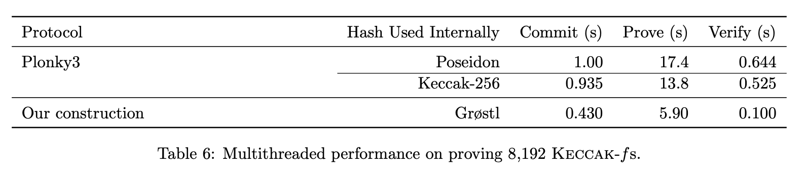
The image above is captured from the **Binius** paper. It turns out Binius is almost 2 times faster to commit, around 2\~3 times faster to prove, and around 5\~6 times faster to verify.

> Written by [Ryan Kim](https://app.gitbook.com/u/cPk8gft4tSd0Obi6ARBfoQ16SqG2 "mention") of Fractalyze

[^1]: ?