# Additive NTT

## Introduction

[**Binius**](https://eprint.iacr.org/2023/1784) is a SNARK constructed using a [**characteristic**](https://en.wikipedia.org/wiki/Characteristic_\(algebra\))**-2** finite field. In Binius, RS-encoding (Reed-Solomon encoding) is employed, but there is a challenge: the conventional Radix-2 FFT cannot be utilized in characteristic-2 finite fields. This paper addresses that challenge.

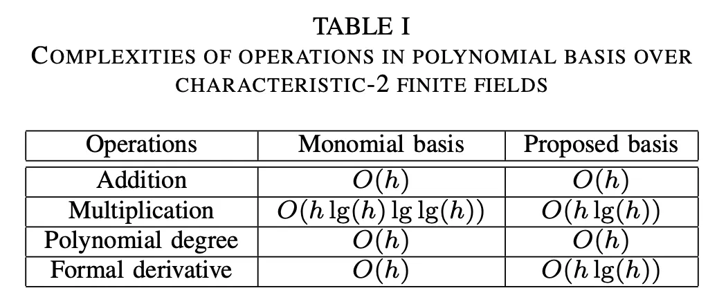
The title of the paper is *"Novel Polynomial Basis and Its Application to Reed-Solomon Erasure Codes."* A characteristic-2 finite field is an extension field of the form $$\mathbb{F}\_{2^r}$$​, which can be constructed as a polynomial ring. Traditionally, polynomials are represented using the Monomial Basis $$1, X, X^2, \dots$$which is a natural choice. However, this paper introduces an ingenious **new polynomial basis** and proposes an encoding algorithm that achieves performance comparable to the Radix-2 FFT.

## Background

### Radix-2 FFT

The **coefficient form** of a univariate polynomial of degree $$n−1$$ is defined as:

$$
P(X) = c\_0 + c\_1X + c\_2X^2 + \cdots + c\_{n-1}X^{n-1}
$$

where the basis is $${1, X, X^2, \dots, X^{n-1}}$$.

On the other hand, the **evaluation form** of a univariate polynomial is defined as:

$$
P(X) = P(x\_0)\cdot L\_0(X) + P(x\_1)\cdot L\_1(X) + P(x\_2)\cdot L\_2(X) + \cdots + P(x\_{n-1})\cdot L\_{n-1}(X)
$$

where the basis is $${L\_0(X), L\_1(X), L\_2(X), \dots, L\_{n-1}(X)}$$, called the **Lagrange basis**.

In **Radix-2 FFT (Fast Fourier Transform)**, a Lagrange basis is constructed using the [roots of unity](https://en.wikipedia.org/wiki/Root_of_unity). Each basis polynomial $$L\_i(X)$$ is defined as:

$$
L\_i(X) = \prod\_{j \ne i}\frac{X - \omega^j}{\omega^i - \omega^j} = \begin{cases} 1 &\text{ if }X = \omega^i \ 0 &\text{ otherwise} \end{cases}
$$

Since we use finite fields instead of complex numbers, this is technically a **Radix-2 NTT (Number Theoretic Transform)**, but for simplicity, we'll refer to it as FFT. Radix-2 FFT transforms a polynomial in coefficient form into its evaluation form. The matrix used to multiply the coefficient vector is called a [**Vandermonde matrix**](https://en.wikipedia.org/wiki/Vandermonde_matrix):

$$
\begin{bmatrix} P(1)\ P(\omega)\ P(\omega^2)\ \vdots \ P(\omega^{n-1}) \end{bmatrix} = \begin{bmatrix} 1 & 1 & 1 & \cdots & 1 \ 1 & \omega & \omega^2 & \cdots & \omega^{n-1} \ 1 & \omega^2 & \omega^4 & \cdots & \omega^{2(n-1)} \ \vdots & \vdots & \vdots & \ddots & \vdots \ 1 & \omega^{n-1} & \omega^{2(n-1)} & \cdots & \omega^{(n-1)^2} \end{bmatrix} \cdot \begin{bmatrix} c\_0 \ c\_1 \ c\_2 \ \vdots \ c\_{n-1} \end{bmatrix}
$$

The $$n$$-th roots of unity satisfy:

$$
\omega^n - 1 = (\omega^{n/2} - 1)(\omega^{n/2} + 1) = 0
$$

Since $$\omega^{n/2}$$ cannot equal $$1$$, it must equal $$-1$$.

Using the property of $$\omega^{n/2} = -1$$, Radix-2 FFT is efficiently computed via the [**Cooley-Tukey algorithm**](https://en.wikipedia.org/wiki/Cooley%E2%80%93Tukey_FFT_algorithm). The polynomial $$P(X)$$ is divided into two parts:

* $$P\_E​(X^2)$$: even powers of $$X$$.
* $$P\_O(X^2)$$: odd powers of $$X$$.

This gives:

$$
P(X) = P\_{E}(X^2) + X \cdot P\_{O}(X^2)
$$

For $$X = -X$$,substituting $$X \cdot \omega^{n/2}$$, we have:

$$
P(-X) = P(X \cdot \omega^{n/2}) = P\_E(X^2) - X\cdot P\_O(X^2)
$$

This transforms an $$n$$-point FFT problem into two $$n / 2$$-point FFT problems.

Define $$\Delta^m\_i(X)$$ as follows:

$$
\Delta^m\_i(X) = \begin{cases} \Delta^m\_{i+1}(X) + X^{2^i}\Delta^{m + 2^i }\_{i+1}(X) & \text{ if }0 \le i < \log\_2 n \ c\_m & \text{ if }i = \log\_2 n\ \end{cases}
$$

For example, for $$n=8$$, the recursive computation proceeds as such:

$$
\begin{align\*} P(X) &= \sum\_{i = 0}^{7}c\_iX\_i \ &= c\_0 + c\_4X^4 + X^2(c\_2 + c\_6X^4) + X(c\_1 + c\_5X^4 + X^2(c\_3 + c\_7X^4)\ &= \Delta^0\_2(X) + X^2\Delta^2\_2(X) + X(\Delta^1\_2(X) + X^2\Delta^3\_2(X)) \ &=\Delta^0\_1(X) + X\Delta^1\_1(X) \ &=\Delta^0\_0(X) \end{align\*}
$$

By recursively applying this process, the computational complexity of FFT becomes $$O(n \cdot \log n)$$.

The **Inverse FFT (IFFT)** converts a polynomial from its evaluation form back to its coefficient form by using the inverse of the **Vandermonde matrix**:

$$
\begin{bmatrix} c\_0 \ c\_1 \ c\_2 \ \vdots \ c\_{n-1} \end{bmatrix} = \begin{bmatrix} 1 & 1 & 1 & \cdots & 1 \ 1 & \omega & \omega^2 & \cdots & \omega^{n-1} \ 1 & \omega^2 & \omega^4 & \cdots & \omega^{2(n-1)} \ \vdots & \vdots & \vdots & \ddots & \vdots \ 1 & \omega^{n-1} & \omega^{2(n-1)} & \cdots & \omega^{(n-1)^2} \end{bmatrix}^{-1} \cdot \begin{bmatrix} P(1)\ P(\omega)\ P(\omega^2)\ \vdots \ P(\omega^{n-1}) \end{bmatrix}
$$

The IFFT can also be computed in $$O(n \cdot \log n)$$ using a similar recursive approach to FFT.

### 2-adicity

When the modulus of a prime field is of the form $$2^S\cdot T + 1$$, a $$2^k$$-th root of unity $$\omega$$ for $$k < S$$ can be determined as follows.

$$
g^{p-1} = g^{2^S \cdot T} = (g^{2^{S-k} \cdot T})^{2^k} = \omega^{2^k} \equiv 1 \pmod p
$$

In other words, if the order of the multiplicative subgroup $$\mathbb{F}\_p^\times$$​ of a prime field is of the form $$2^S \cdot T$$, and $$S$$ (also known as the **2-adicity**) is large, FFT can be used effectively. Fields with this structure are referred to as **FFT-friendly fields**.

What about characteristic-2 finite fields, such as $$\mathbb{F}*{2^r}$$​? For these fields, the order of the multiplicative subgroup $$\mathbb{F}*{2^r}^{\times}$$ is $$2^r - 1$$. Since the 2-adicity of $$2^r - 1$$ is 0, Radix-2 FFT cannot be used.

This naturally raises the question: when the characteristic is 2, what new polynomial basis would be suitable? Moreover, to achieve fast computation similar to Radix-2 FFT, the method must recursively reduce the problem into smaller subproblems.Protocol Explanation

**NOTE:** From this point onward, $$\omega$$ is no longer a root of unity, and $$\Delta$$ will be newly defined.

### Polynomial Basis

The elements of $$\mathbb{F}*{2^r}$$ can be represented as the set $${\omega\_i}*{i=0}^{2^r - 1}$$, where:

$$
i = \sum\_{k = 0}^{r-1}i\_k \cdot 2^k, \forall i\_k \in {0,1}
$$

Given a basis vector $$v = {v\_0, \dots, v\_{r-1}}$$ composed of elements from $$\mathbb{F}\_{2^r}$$, each $$\omega\_i$$ can be expressed as:

$$
\omega\_i = \sum\_{k = 0}^{r-1}i\_k \cdot v\_k
$$

We define the **subspace vanishing polynomial** as:

$$
W\_j(X) = \prod\_{i=0}^{2^j-1}(X + \omega\_i)\text{, where } 0 \le j \le r - 1
$$

This mean the full form of the vanishing polynomials $$W\_j(X)$$ are as follows:

$$
W\_0(X) = X + \omega\_0, \ W\_1(X) = (X + \omega\_0)(X + \omega\_1) ,\ W\_2(X) = (X + \omega\_0)(X + \omega\_1)(X + \omega\_2)(X + \omega\_3) ,\\
$$

and so on.

Thus, $$\deg(W\_j(X)) = 2^j$$ and the roots of $$W\_2(X)$$ are $$\omega\_0, \omega\_1, \omega\_2, \omega\_3$$ . This follows from the fact that addition in $$\mathbb{F}\_{2^r}$$​ is XOR, so $$\omega\_i + \omega\_i = 0$$, a direct result of the field’s characteristic being 2.

**Lemma 1.** $$W\_j(X)$$ is a $$\mathbb{F}\_2$$-linearized polynomial.

$$
W\_j(X) = \sum\_{i = 0}^{j}a\_{j,i}X^{2^i} \text{, where }a\_{j,i} \in \mathbb{F}\_{2^r}
$$

Furthermore, $$W\_j(X)$$ satisfies the following property:

$$
W\_j(X + Y) = W\_j(X) + W\_j(Y), \forall X,Y \in \mathbb{F}\_{2^r}
$$

We now define a new **polynomial basis** $$X\_i(X)$$ as:

$$
X\_i(X) = \prod\_{j= 0}^{r-1}(\frac{W\_j(X)}{W\_j(\omega\_{2^j})})^{i\_j}
$$

where:

$$
i = \sum\_{j = 0}^{r-1}i\_j \cdot 2^j, \forall i\_j \in {0,1}
$$

The new polynomial basis $$X\_i(X)$$ is as follows:

$$
X\_0(X) = 1 ,
\ X\_1(X) = \frac{W\_0(X)}{W\_0(\omega\_1)} = \frac{X + \omega\_0}{\omega\_1 + \omega\_0} ,
\ X\_2(X) = \frac{W\_1(X)}{W\_1(\omega\_2)} = \frac{(X + \omega\_0)(X + \omega\_1)}{(\omega\_2 + \omega\_0)(\omega\_2 + \omega\_1)},
\ X\_3(X) = \frac{W\_0(X)W\_1(X)}{W\_0(\omega\_1)W\_1(\omega\_2)} = \frac{(X + \omega\_0)^2(X + \omega\_1)}{(\omega\_1 + \omega\_0)(\omega\_2 + \omega\_0)(\omega\_2 + \omega\_1)} ,
\ X\_4(X) = \frac{W\_2(X)}{W\_2(\omega\_4)} = \frac{(X + \omega\_0)(X + \omega\_1)(X + \omega\_2)(X + \omega\_3)}{(\omega\_4 + \omega\_0)(\omega\_4 + \omega\_1)(\omega\_4 + \omega\_2)(\omega\_4 + \omega\_3)},
$$

and so on.

Thus, $$\deg(X\_i(X)) = i$$.

The **coefficient form** of an $$n-1$$-degree univariate polynomial $$[D\_n](https://fractalyze.gitbook.io/intro/~/revisions/0AAov1j5GF4J6Ca62R1w/zk/stark/X) \in \mathbb{F}\_{2^r}\[X] / (X^{2^r} - 1)$$ is expressed as:

$$
[D\_n](https://fractalyze.gitbook.io/intro/~/revisions/0AAov1j5GF4J6Ca62R1w/zk/stark/X) = d\_0 + d\_1X\_1(X) + d\_2X\_2(X) + \dots + d\_{n-1}X\_{n-1}(X)
$$

The **evaluation form** of this polynomial is:

$$
[D\_n](https://fractalyze.gitbook.io/intro/~/revisions/0AAov1j5GF4J6Ca62R1w/zk/stark/X) = \[D\_n]\(\omega\_0 + \omega\_l) \cdot L^l\_0(X) + \[D\_n]\(\omega\_1 + \omega\_l) \cdot L^l\_1(X) + \[D\_n]\(\omega\_2 + \omega\_l) \cdot L^l\_2(X) + \cdots + \[D\_n]\(\omega\_{n-1} + \omega\_l) \cdot L^l\_{n-1}(X)
$$

where $$L^l\_i(X)$$ is defined as:

$$
L^l\_i(X) = \prod\_{j \ne i}\frac{X - \omega\_j}{\omega\_i + \omega\_l - \omega\_j} = \begin{cases} 1 &\text{ if }X = \omega\_i + \omega\_l \ 0 &\text{ otherwise} \end{cases}
$$

We denote the set of evaluations as $$\hat{D}^l\_n$$, defined as such:

$$
\hat{D}^l\_n = {\[D\_n]\(\omega\_0 + \omega\_l), \[D\_n]\(\omega\_1 + \omega\_l),\[D\_n]\(\omega\_2 + \omega\_l),\dots, \[D\_n]\(\omega\_{n-1} + \omega\_l) }
$$

### Delta Polynomial

The recursive calculation of $$[D\_n](https://fractalyze.gitbook.io/intro/~/revisions/0AAov1j5GF4J6Ca62R1w/zk/stark/X)$$ can be performed by defining $$\Delta^m\_i(X)$$ as follows:

$$
\Delta^m\_i(X) = \begin{cases}
\Delta^m\_{i+1}(X) + \frac{W\_i(X)}{W\_i(\omega\_{2^i})}\Delta^{m + 2^i}\_{i+1}(X) & \text{ if }0 \le i < \log\_2 n \\
d\_m & \text { if } i = \log\_2n \end{cases}
$$

where $$0 \le m < 2^i$$.

For $$n = 8$$, $$\Delta$$ exists as follows:

$$
\Delta^0\_3(X) = d\_0,\Delta^1\_3(X) = d\_1, \Delta^2\_3(X) = d\_2, \dots, \Delta^7\_3(X) = d\_7, \\
\Delta^0\_2(X) = \Delta^0\_3(X) + \frac{W\_2(X)}{W\_2(\omega\_4)} \Delta^4\_3(X) = d\_0 + \frac{W\_2(X)}{W\_2(\omega\_4)}d\_4, \\
\Delta^1\_2(X) = \Delta^1\_3(X) + \frac{W\_2(X)}{W\_2(\omega\_4)} \Delta^5\_3(X) = d\_1 + \frac{W\_2(X)}{W\_2(\omega\_4)}d\_5, \\
\Delta^2\_2(X) = \Delta^2\_3(X) + \frac{W\_2(X)}{W\_2(\omega\_4)} \Delta^6\_3(X) = d\_2 + \frac{W\_2(X)}{W\_2(\omega\_4)}d\_6, \\
\Delta^3\_2(X) = \Delta^3\_3(X) + \frac{W\_2(X)}{W\_2(\omega\_4)} \Delta^7\_3(X) = d\_3 + \frac{W\_2(X)}{W\_2(\omega\_4)}d\_7, \\
\Delta^0\_1(X) = \Delta^0\_2(X) + \frac{W\_1(X)}{W\_1(\omega\_2)} \Delta^2\_2(X), \\
\Delta^1\_1(X) = \Delta^1\_2(X) + \frac{W\_1(X)}{W\_1(\omega\_2)} \Delta^3\_2(X), \\
\Delta^0\_0(X) = \Delta^0\_1(X) + \frac{W\_0(X)}{W\_0(\omega\_1)} \Delta^1\_1(X)
$$

$$[D\_n](https://fractalyze.gitbook.io/intro/~/revisions/0AAov1j5GF4J6Ca62R1w/zk/stark/X)$$ is equivalent to $$\Delta^0\_0(X)$$. For example, $$[D\_8](https://fractalyze.gitbook.io/intro/~/revisions/0AAov1j5GF4J6Ca62R1w/zk/stark/X)$$ is recursively computed as follows:

$$
\begin{align\*} [D\_8](https://fractalyze.gitbook.io/intro/~/revisions/0AAov1j5GF4J6Ca62R1w/zk/stark/X) &= \sum\_{i = 0}^{7} d\_iX\_i(X) \ &=d\_0 + d\_1\frac{W\_0(X)}{W\_0(\omega\_1)} + d\_2\frac{W\_1(X)}{W\_1(\omega\_2)} + d\_3\frac{W\_0(X)W\_1(X)}{W\_0(\omega\_1)W\_1(\omega\_2)} + d\_4\frac{W\_2(X)}{W\_2(\omega\_4)} \ &\space\space\space\space\space d\_5\frac{W\_0(X)W\_2(X)}{W\_0(\omega\_1)W\_2(\omega\_4)} + d\_6\frac{W\_1(X)W\_2(X)}{W\_1(\omega\_2)W\_2(\omega\_4)} + d\_7\frac{W\_0(X)W\_1(X)W\_2(X)}{W\_0(\omega\_1)W\_1(\omega\_2)W\_2(\omega\_4)} \ &=\bigg(d\_0 + d\_4\frac{W\_2(X)}{W\_2(\omega\_4)} + \frac{W\_1(X)}{W\_1(\omega\_2)}\bigg( d\_2 + d\_6\frac{W\_2(X)}{W\_2(\omega\_4)}\bigg)\bigg) \ &\space\space\space\space\space + \frac{W\_0(X)}{W\_0(\omega\_1)}\bigg(d\_1 + d\_5\frac{W\_2(X)}{W\_2(\omega\_4)} + \frac{W\_1(X)}{W\_1(\omega\_2)}\bigg(d\_3 + d\_7\frac{W\_2(X)}{W\_2(\omega\_4)} \bigg) \bigg) \ &=\bigg(\Delta^0\_2(X) + \frac{W\_1(X)}{W\_1(\omega\_2)}\Delta^2\_2(X) \bigg) + \frac{W\_0(X)}{W\_0(\omega\_1)}\bigg( \Delta^1\_2(X) + \frac{W\_1(X)}{W\_1(\omega\_2)}\Delta^3\_2(X) \bigg) \ &= \Delta^0\_1(X) + \frac{W\_0(X)}{W\_0(\omega\_1)}\Delta^1\_1(X) \ &= \Delta^0\_0(X) \end{align\*}
$$

**Lemma 2.** $$\Delta^m\_i(X + Y) = \Delta^m\_i(X), \forall Y \in {\omega\_b}\_{b = 0}^{2^i - 1}$$

**Proof:**

**Case 1:** $$i = \log\_2 n$$, both $$\Delta^m\_i(X + Y)$$ and $$\Delta^m\_i(X)$$ equal $$d\_m$$, so the equality holds trivially.

**Case 2:** $$i = \log\_2 n - 1$$, $$\Delta^m\_i(X)$$ is given as:

$$
\begin{align\*} \Delta^m\_{\log\_2 n - 1}(X) &= \Delta^m\_{\log\_2 n}(X) + \frac{W\_{\log\_2 n - 1}(X)}{W\_{\log\_2 n - 1}(\omega\_{2^{\log\_2 n - 1}})} \Delta^{m + 2^{\log\_2 n - 1}}*{\log\_2 n}(X) \\
&= d\_m + \frac{W*{\log\_2 n - 1}(X)}{W\_{\log\_2 n - 1}(\omega\_{2^{\log\_2 n - 1}})} d\_{m + 2^{\log\_2 n - 1}} \end{align\*}
$$

which simplifies as follows:

$$
\Delta^m\_{\log\_2 n - 1}(X + Y)
\= d\_m + \frac{W\_{\log\_2 n - 1}(X + Y)}{W\_{\log\_2 n - 1}(\omega\_{2^{\log\_2 n - 1}})} d\_{m + 2^{\log\_2 n - 1}}
$$

Using **Lemma 1**:

$$
W\_{\log\_2 n - 1}(X + Y) = W\_{\log\_2 n - 1}(X) + W\_{\log\_2 n - 1}(Y)
$$

Since $$Y \in {\omega\_b}*{b=0}^{2^i - 1}$$, we know $$W*{\log\_2 n - 1}(Y) = 0$$, so:

$$
\begin{align\*}
\Delta^m\_{\log\_2 n - 1}(X + Y)
&= d\_m + \frac{W\_{\log\_2 n - 1}(X)}{W\_{\log\_2 n - 1}(\omega\_{2^{\log\_2 n - 1}})} d\_{m + 2^{\log\_2 n - 1}} \\
&= \Delta^m\_{\log\_2 n -1}(X)
\end{align\*}
$$

**Case 3:** Inductive Step

Assume the equality holds for $$i = c+ 1$$. At , we have:

$$
\Delta^m\_{c}(X + Y)  = \Delta^m\_{c + 1}(X + Y) + \frac{W\_{c}(X + Y)}{W\_{c}(\omega\_{2^c})} \Delta^{m + 2^c}\_{c + 1}(X + Y)
$$

By **Lemma 1**:

$$
W\_c(X + Y) = W\_c(X) + W\_c(Y)
$$

Since $$Y \in {\omega\_b}*{b=0}^{2^c - 1}$$, we know $$W*{c}(Y) = 0$$, thus:

$$
\begin{align\*}
\Delta^m\_{c}(X + Y)  &= \Delta^m\_{c + 1}(X + Y) + \frac{W\_{c}(X)}{W\_{c}(\omega\_{2^c})} \Delta^{m + 2^c}\_{c + 1}(X + Y)  \\
&= \Delta^m\_c(X)
\end{align\*}
$$

### Transform

Define the transform $$\Psi$$ as:

$$
\Psi(i, m, l) = \begin{cases} { \Delta^m\_i(\omega\_c + \omega\_l)| c \in {b \cdot 2^i}^{n/2^i - 1}\_{b = 0} } & \text{ if } 0 \le i < \log\_2 n \ {d\_m} & \text{ if } i = \log\_2n \end{cases}
$$

where $$0 \le m < 2^i$$.

The transform computes $${\Psi(\log\_2 n, k, l)|k \in \[0, n-1]} \rightarrow \Psi(0, 0, l)$$. For $$n = 8$$, this becomes:

$$
{d\_0, d\_1, d\_2 \dots, d\_{7}} = \Psi(3, 0, l) \cup \Psi(3, 1, l) \cup \Psi(3, 2, l) \cup \cdots \cup \Psi(3, 7, l) \ \rightarrow {\Delta^0\_0(\omega\_0 + \omega\_l),\Delta^0\_0(\omega\_1 + \omega\_l), \Delta^0\_0(\omega\_2 + \omega\_l), \dots, \Delta^0\_0(\omega\_{7} + \omega\_l)} = \Psi(0, 0, l)
$$

Remember that $$\Delta^0\_0(X)$$ is equivalent to $$[D\_n](https://fractalyze.gitbook.io/intro/~/revisions/0AAov1j5GF4J6Ca62R1w/zk/stark/X)$$.

$$\Psi(i, m, l)$$ can be divided into two parts as follows:

* $${\Delta^m\_i(\omega\_c + \omega\_l)| c \in {b \cdot 2^{i+1}}^{n/2^{i+1} - 1}\_{b = 0}}$$ which can be computed from $$\Psi(i + 1, m, l)$$.
* $${\Delta^m\_i(\omega\_c + \omega\_l + \omega\_{2^i})| c \in {b \cdot 2^{i+1}}^{n/2^{i+1} - 1}\_{b = 0}}$$ which can be computed from $$\Psi(i + 1, m +2^i, l)$$.

**Part 1.** $$\Psi(i + 1, m, l)$$

$$
\Delta^m\_i(\omega\_c + \omega\_l) = \Delta^m\_{i+1}(\omega\_c + \omega\_l) + \frac{W\_i(\omega\_c + \omega\_l)}{W\_i(\omega\_{2^i})}\Delta^{m + 2^i}\_{i +1}(\omega\_c + \omega\_l)
$$

Since all the right-hand terms are known, the left-hand terms can be determined.

**Part 2.** $$\Psi(i + 1, m + 2^i, l)$$

$$
\begin{align\*}
\Delta^m\_i(\omega\_c + \omega\_l + \omega\_{2^i}) &= \Delta^m\_{i+1}(\omega\_c + \omega\_l + \omega\_{2^i}) + \frac{W\_i(\omega\_c + \omega\_l + \omega\_{2^i})}{W\_i(\omega\_{2^i})}\Delta^{m + 2^i}*{i +1}(\omega\_c + \omega\_l + \omega{2^i})
\ &= \Delta^m*{i+1}(\omega\_c + \omega\_l) + \frac{W\_i(\omega\_c + \omega\_l + \omega\_{2^i})}{W\_i(\omega\_{2^i})}\Delta^{m + 2^i}*{i +1}(\omega\_c + \omega\_l) \because \text{Lemma } 2.
\ &= \Delta^m*{i+1}(\omega\_c + \omega\_l) + \frac{W\_i(\omega\_c + \omega\_l) + W\_i(\omega\_{2^i})}{W\_i(\omega\_{2^i})}\Delta^{m + 2^i}*{i +1}(\omega\_c + \omega\_l) \because \text{Lemma } 1.
\ &= \Delta^m*{i+1}(\omega\_c + \omega\_l) + \frac{W\_i(\omega\_c + \omega\_l)}{W\_i(\omega\_{2^i})}\Delta^{m + 2^i}*{i +1}(\omega\_c + \omega\_l) + \Delta^{m + 2^i}*{i +1}(\omega\_c + \omega\_l)
\ &= \Delta^m\_i(\omega\_c + \omega\_l) + \Delta^{m + 2^i}\_{i+1}(\omega\_c + \omega\_l) \end{align\*}
$$

Since $$\Delta^m\_i(\omega\_c + \omega\_l)$$ can be computed from the Part 1, the left-hand terms can be determined.

When $$n=8, i=2$$, for $$\Psi(2, m, l)$$, it can be split into $$\Psi(3,m , l) = {d\_m}$$ and $$\Psi(3, m + 4, l) = \Delta^{m+4}*3(X) ={d*{m+4}}$$.

$$
\begin{align\*}
\Psi(2, m, l) &= {\Delta^m\_2(\omega\_0 + \omega\_l),\Delta^m\_2(\omega\_4 + \omega\_l)}
\ &= {\Delta^m\_3(\omega\_0 + \omega\_l) + \frac{W\_2(\omega\_0 + \omega\_l)}{W\_2(\omega\_4)}\Delta^{m + 4}*3(\omega\_0 + \omega\_l), \Delta^m\_3(\omega\_4 + \omega\_l) + \frac{W\_2(\omega\_4 + \omega\_l)}{W\_2(\omega\_4)}\Delta^{m + 4}*3(\omega\_4 + \omega\_l) }
\ &= {d\_m + \frac{W\_2(\omega\_0 + \omega\_l)}{W\_2(\omega\_4)}d*{m+4}, d\_m + \frac{W\_2(\omega\_4 + \omega\_l)}{W\_2(\omega\_4)}d*{m+4} }
\end{align\*}
$$

When $$n=8, i=1$$, for $$\Psi(1, m, l)$$, it can be split into$$\Psi(2, m, l) = {\Delta^m\_2(\omega\_0 + \omega\_l), \Delta^m\_2(\omega\_4 + \omega\_l)}$$ and $$\Psi(2, m + 2, l) = {\Delta^{m + 2}\_2(\omega\_0 + \omega\_l), \Delta^{m + 2}\_2(\omega\_4 + \omega\_l)}$$.

$$
\begin{align\*}\Psi(1, m, l) &= {\Delta^m\_1(\omega\_0 + \omega\_l),\Delta^m\_1(\omega\_2 + \omega\_l),\Delta^m\_1(\omega\_4 + \omega\_l),\Delta^m\_1(\omega\_6 + \omega\_l)} \ &= {\Delta^m\_2(\omega\_0 + \omega\_l) + \frac{W\_1(\omega\_0 + \omega\_l)}{W\_1(\omega\_2)}\Delta^{m + 2}\_2(\omega\_0 + \omega\_l), \Delta^m\_2(\omega\_2 + \omega\_l) + \frac{W\_1(\omega\_2 + \omega\_l)}{W\_1(\omega\_2)}\Delta^{m + 2}\_2(\omega\_2 + \omega\_l), \Delta^m\_2(\omega\_4 + \omega\_l) + \frac{W\_1(\omega\_4 + \omega\_l)}{W\_1(\omega\_2)}\Delta^{m + 2}\_2(\omega\_4 + \omega\_l), \Delta^m\_2(\omega\_6 + \omega\_l) + \frac{W\_1(\omega\_6 + \omega\_l)}{W\_1(\omega\_2)}\Delta^{m + 2}\_2(\omega\_6 + \omega\_l) } \ &= {\Delta^m\_2(\omega\_0 + \omega\_l) + \frac{W\_1(\omega\_0 + \omega\_l)}{W\_1(\omega\_2)}\Delta^{m + 2}\_2(\omega\_0 + \omega\_l), \Delta^m\_2(\omega\_0 + \omega\_l + \omega\_2) + \frac{W\_1(\omega\_0 + \omega\_l + \omega\_2)}{W\_1(\omega\_2)}\Delta^{m + 2}\_2(\omega\_0 + \omega\_l + \omega\_2), \Delta^m\_2(\omega\_4 + \omega\_l) + \frac{W\_1(\omega\_4 + \omega\_l)}{W\_1(\omega\_2)}\Delta^{m + 2}\_2(\omega\_4 + \omega\_l), \Delta^m\_2(\omega\_4 + \omega\_l + \omega\_2) + \frac{W\_1(\omega\_4 + \omega\_l + \omega\_2)}{W\_1(\omega\_2)}\Delta^{m + 2}\_2(\omega\_4 + \omega\_l + \omega\_2) } \ &= {\Delta^m\_2(\omega\_0 + \omega\_l) + \frac{W\_1(\omega\_0 + \omega\_l)}{W\_1(\omega\_2)}\Delta^{m + 2}\_2(\omega\_0 + \omega\_l), \Delta^m\_2(\omega\_0 + \omega\_l) + \frac{W\_1(\omega\_0 + \omega\_l)}{W\_1(\omega\_2)}\Delta^{m + 2}\_2(\omega\_0 + \omega\_l), \Delta^m\_2(\omega\_4 + \omega\_l) + \frac{W\_1(\omega\_4 + \omega\_l)}{W\_1(\omega\_2)}\Delta^{m + 2}\_2(\omega\_4 + \omega\_l), \Delta^m\_2(\omega\_4 + \omega\_l) + \frac{W\_1(\omega\_4 + \omega\_l)}{W\_1(\omega\_2)}\Delta^{m + 2}\_2(\omega\_4 + \omega\_l) } \ \end{align\*}
$$

### Inverse Transform

To compute $$\Psi(i + 1, m, l)$$ and $$\Psi(i + 1, m + 2^i, l)$$ from $$\Psi(i, m, l)$$:

**Part 1.** $$\Psi(i + 1, m + 2^i, l)$$

$$
\Psi(i + 1, m + 2^i, l) = {\Delta^{m + 2^i}*{i+1}(\omega\_c + \omega\_l)| c \in {b \cdot 2^{i+1}}^{n/2^{i+1} - 1}*{b = 0}}
$$

where: (Refer to Part 2. in Transform section above.)

$$
\Delta^{m + 2^i}*{i+1}(\omega\_c + \omega\_l) = \Delta^m\_i(\omega\_c + \omega\_l) + \Delta^m\_i(\omega\_c + \omega\_l + \omega*{2^i})
$$

Since all the right-hand terms are known, the left-hand terms can be determined.

**Part 2.** $$\Psi(i + 1, m, l)$$

$$
\Psi(i + 1, m, l) = {\Delta^{m }*{i+1}(\omega\_c + \omega\_l)| c \in {b \cdot 2^{i+1}}^{n/2^{i+1} - 1}*{b = 0}}
$$

where (Refer to Part 1. in Transform section above):

$$
\Delta^{m}*{i+1}(\omega\_c + \omega\_l) = \Delta^m\_i(\omega\_c + \omega\_l) + \frac{W\_i(\omega\_c + \omega\_l)}{W\_i(\omega*{2^i})}\Delta^{m + 2^i}\_{i+1}(\omega\_c + \omega\_l)
$$

Since $$\Delta^m\_i(\omega\_c + \omega\_l)$$ can be computed from the Part 1, the left-hand terms can be determined.

<figure><img src="https://755218234-files.gitbook.io/~/files/v0/b/gitbook-x-prod.appspot.com/o/spaces%2Frwz1ZAZJtK5FHz4Y1esA%2Fuploads%2Fgit-blob-5d684787cdc9833c5ee36c5ebd73ee0d9d8e377f%2Fimage.png?alt=media" alt=""><figcaption></figcaption></figure>

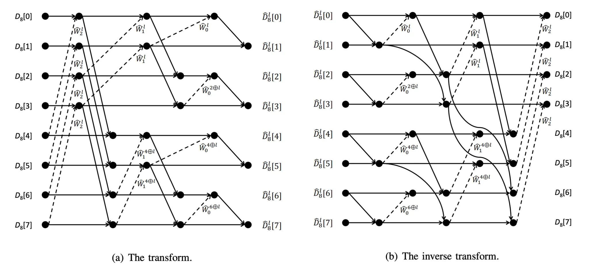
The diagram above illustrates the data dependencies for transforming and inversely transforming a polynomial of size 8. Each eleme[nt is computed as the sum of a solid-line element and a dashed-line element, where the la](#user-content-fn-1)[^1]tter represents scalar multiplication by $$\widehat{W}^j\_i$$.

$$
\widehat{W}^j\_i = \frac{W\_i(\omega\_j)}{W\_i(\omega\_{2^i})}
$$

## Conclusion

The method for performing a formal derivative on the **Novel Polynomial Basis** and its use in the RS erasure decoding algorithm is omitted here due to space constraints. For those interested, please refer to the original paper.

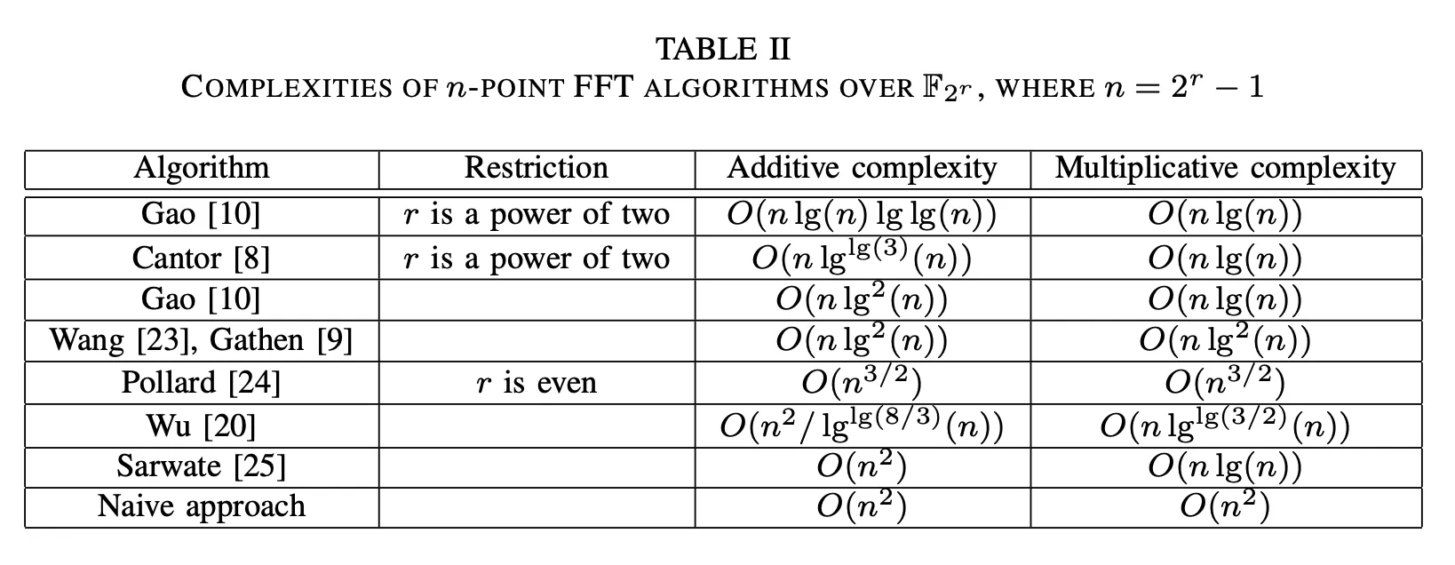
<figure><img src="https://755218234-files.gitbook.io/~/files/v0/b/gitbook-x-prod.appspot.com/o/spaces%2Frwz1ZAZJtK5FHz4Y1esA%2Fuploads%2Fgit-blob-357d8be692c288a92f1759e258909913a2e6247e%2Fimage.png?alt=media" alt=""><figcaption><p>Complexities of Previous n-point FFT Algorithms</p></figcaption></figure>

Using the newly proposed Novel Polynomial Basis, the Additive NTT achieves $$O(n \log n)$$ additive complexity and $$O(n \log n)$$ multiplicative complexity without any constraints. Consequently, for the first time, RS-encoding over characteristic-2 finite fields achieves $$O(n \log n)$$ complexity.

<figure><img src="https://755218234-files.gitbook.io/~/files/v0/b/gitbook-x-prod.appspot.com/o/spaces%2Frwz1ZAZJtK5FHz4Y1esA%2Fuploads%2Fgit-blob-9322ef38e6f45ee41a6a60a049f9d937d907da22%2Fimage.png?alt=media" alt=""><figcaption></figcaption></figure>

Additionally, it is well-known that polynomial multiplication can be optimized using FFT. Similarly, by leveraging the Novel Polynomial Basis, multiplication in characteristic-2 finite fields can also be optimized.

> Written by [Ryan Kim](https://app.gitbook.com/u/cPk8gft4tSd0Obi6ARBfoQ16SqG2 "mention") of Fractalyze

[^1]: n